Avijit Podder Date: Feb 26, 2025

library(stringr)
library(dplyr)

## 
## Attaching package: 'dplyr'

## The following objects are masked from 'package:stats':
## 
##     filter, lag

## The following objects are masked from 'package:base':
## 
##     intersect, setdiff, setequal, union

library(viridis)

## Loading required package: viridisLite

library(gplots)

## 
## Attaching package: 'gplots'

## The following object is masked from 'package:stats':
## 
##     lowess

library(ggplot2)

## Warning: package 'ggplot2' was built under R version 4.5.2

library(reshape2)
library(RColorBrewer)
library(ggrepel)
library(tidyr)

## 
## Attaching package: 'tidyr'

## The following object is masked from 'package:reshape2':
## 
##     smiths

library(DT)
library(patchwork)
library(corrplot)

## corrplot 0.95 loaded

library(plotly)

## 
## Attaching package: 'plotly'

## The following object is masked from 'package:ggplot2':
## 
##     last_plot

## The following object is masked from 'package:stats':
## 
##     filter

## The following object is masked from 'package:graphics':
## 
##     layout

library(htmlwidgets)
library(qvalue)


# Open sample information file as "sample_data" for TMT specific 610 samples (round 1 and round2)
sample_data <- read.csv("2c.traits-ROSMAP610.R1+R2-2xTAMPORcorrected.csv", sep =",", header = TRUE, stringsAsFactors = FALSE)

dim(sample_data)

## [1] 610  40

head(sample_data)

##   batch.channel projid.ROSMAP study.ROSMAP scaled_to.ROSMAP apoe_genotype
## 1      b01.127N      20271359         ROS            ROSMAP           e33
## 2      b01.127C      33477756         MAP            ROSMAP           e33
## 3      b01.128N      38967303         MAP            ROSMAP           e33
## 4      b01.128C      10100736         ROS            ROSMAP           e34
## 5      b01.129N      10298957         ROS            ROSMAP           e33
## 6      b01.129C      46291609         MAP            ROSMAP           e33
##   ApoE4.Dose ApoE.Risk age_first_ad_dx cogdx cogdx_stroke dxpark cogn_global_lv
## 1          0         0           90.00     4            2      2          -0.36
## 2          0         0              NA     1            2      2           0.00
## 3          0         0              NA     1            1      2           0.45
## 4          1         1              NA     1            2      2           0.39
## 5          0         0           81.65     4            2      1          -1.63
## 6          0         0              NA     2            2      2          -0.08
##   cts_mmse30_lv age_death educ msex race7 braaksc ceradsc_RADCnonStd gpath
## 1            25     90.00   18    0     1       4                  2  0.24
## 2            28     90.00   16    0     1       3                  2  0.71
## 3            28     84.83   11    0     1       3                  4  0.09
## 4            28     90.00   14    1     1       4                  3  0.34
## 5            10     82.37   24    1     1       3                  2  0.85
## 6            24     87.59   14    0     1       4                  2  0.89
##   niareagansc   pmi amyloid amyloid_mf dlbdx mglia123_mf mglia23_mf mglia3_mf
## 1           2 18.33    1.17       1.42     2          NA         NA        NA
## 2           2  4.77    5.40       7.87     2          NA         NA        NA
## 3           3  6.50    0.00       0.00     0      170.35       3.91         0
## 4           3 15.17    2.47       5.06     0          NA         NA        NA
## 5           2  3.93    8.49      13.82     3          NA         NA        NA
## 6           2  7.42    7.78      18.42     0          NA         NA        NA
##    nft tangles tangles_mf tdp_cs_6reg tdp_st4 brainwt CERAD JohnsonDx
## 1 0.44    3.55       0.02        1.83       2    1138     2    AsymAD
## 2 0.17    2.07       0.00        0.67       1    1110     2    AsymAD
## 3 0.28    3.02       0.00        0.17       1    1250     0   Control
## 4 0.71    4.95       0.00        0.00       0    1130     1    AsymAD
## 5 0.43    5.12       0.00        0.00       0    1300     2        AD
## 6 0.48    3.40       0.03        0.00       0    1192     2    AsymAD
##           Batch  GIS BatchColor                         tissue
## 1 ROSMAP.R1.400 <NA>  turquoise dorsolateral prefrontal cortex
## 2 ROSMAP.R1.400 <NA>  turquoise dorsolateral prefrontal cortex
## 3 ROSMAP.R1.400  GIS  turquoise dorsolateral prefrontal cortex
## 4 ROSMAP.R1.400 <NA>  turquoise dorsolateral prefrontal cortex
## 5 ROSMAP.R1.400 <NA>  turquoise dorsolateral prefrontal cortex
## 6 ROSMAP.R1.400 <NA>  turquoise dorsolateral prefrontal cortex

# Define the sex_type (sex) based on the msex value
sample_data$sex <- with(sample_data, ifelse(msex == 0, "female",
                                ifelse(msex == 1, "male", "NA")))

# Create a new categorical column based on cts_mmse30_lv
sample_data$cts_mmse30_cat <- ifelse(sample_data$cts_mmse30_lv <= 23, "0", "1")



dim(sample_data)

## [1] 610  42

head(sample_data)

##   batch.channel projid.ROSMAP study.ROSMAP scaled_to.ROSMAP apoe_genotype
## 1      b01.127N      20271359         ROS            ROSMAP           e33
## 2      b01.127C      33477756         MAP            ROSMAP           e33
## 3      b01.128N      38967303         MAP            ROSMAP           e33
## 4      b01.128C      10100736         ROS            ROSMAP           e34
## 5      b01.129N      10298957         ROS            ROSMAP           e33
## 6      b01.129C      46291609         MAP            ROSMAP           e33
##   ApoE4.Dose ApoE.Risk age_first_ad_dx cogdx cogdx_stroke dxpark cogn_global_lv
## 1          0         0           90.00     4            2      2          -0.36
## 2          0         0              NA     1            2      2           0.00
## 3          0         0              NA     1            1      2           0.45
## 4          1         1              NA     1            2      2           0.39
## 5          0         0           81.65     4            2      1          -1.63
## 6          0         0              NA     2            2      2          -0.08
##   cts_mmse30_lv age_death educ msex race7 braaksc ceradsc_RADCnonStd gpath
## 1            25     90.00   18    0     1       4                  2  0.24
## 2            28     90.00   16    0     1       3                  2  0.71
## 3            28     84.83   11    0     1       3                  4  0.09
## 4            28     90.00   14    1     1       4                  3  0.34
## 5            10     82.37   24    1     1       3                  2  0.85
## 6            24     87.59   14    0     1       4                  2  0.89
##   niareagansc   pmi amyloid amyloid_mf dlbdx mglia123_mf mglia23_mf mglia3_mf
## 1           2 18.33    1.17       1.42     2          NA         NA        NA
## 2           2  4.77    5.40       7.87     2          NA         NA        NA
## 3           3  6.50    0.00       0.00     0      170.35       3.91         0
## 4           3 15.17    2.47       5.06     0          NA         NA        NA
## 5           2  3.93    8.49      13.82     3          NA         NA        NA
## 6           2  7.42    7.78      18.42     0          NA         NA        NA
##    nft tangles tangles_mf tdp_cs_6reg tdp_st4 brainwt CERAD JohnsonDx
## 1 0.44    3.55       0.02        1.83       2    1138     2    AsymAD
## 2 0.17    2.07       0.00        0.67       1    1110     2    AsymAD
## 3 0.28    3.02       0.00        0.17       1    1250     0   Control
## 4 0.71    4.95       0.00        0.00       0    1130     1    AsymAD
## 5 0.43    5.12       0.00        0.00       0    1300     2        AD
## 6 0.48    3.40       0.03        0.00       0    1192     2    AsymAD
##           Batch  GIS BatchColor                         tissue    sex
## 1 ROSMAP.R1.400 <NA>  turquoise dorsolateral prefrontal cortex female
## 2 ROSMAP.R1.400 <NA>  turquoise dorsolateral prefrontal cortex female
## 3 ROSMAP.R1.400  GIS  turquoise dorsolateral prefrontal cortex female
## 4 ROSMAP.R1.400 <NA>  turquoise dorsolateral prefrontal cortex   male
## 5 ROSMAP.R1.400 <NA>  turquoise dorsolateral prefrontal cortex   male
## 6 ROSMAP.R1.400 <NA>  turquoise dorsolateral prefrontal cortex female
##   cts_mmse30_cat
## 1              1
## 2              1
## 3              1
## 4              1
## 5              0
## 6              1

##################################################################################################################################################

# Select a sub-set of the sample (Tissue: DLPFC) from sample_data file
sample_data_DLPFC <- filter(sample_data, tissue == "dorsolateral prefrontal cortex")

dim(sample_data_DLPFC)

## [1] 610  42

# Read the outliers file
outliers <- read.table("outliers.txt", header = TRUE)

# Extract the IDs to be removed
ids_to_remove <- outliers$Outliers

ids_to_remove

## [1] "b22.130N" "b52.130N"

# Use the 'subset' function to remove rows with specified IDs (outliers) from the sample description file with CT samples
sample_data_DLPFC <- subset(sample_data_DLPFC, !(batch.channel %in% ids_to_remove))

dim(sample_data_DLPFC)

## [1] 608  42

##################################################################################################################################################

# Create a subset of the DLPFC sample description file with control samples only
sample_data_DLPFC_contorl <- sample_data_DLPFC[grep("Control", sample_data_DLPFC$JohnsonDx), ]

dim(sample_data_DLPFC_contorl)

## [1] 114  42

# Create a subset of the control sample description file with female samples only
#sample_data_DLPFC_contorl_female <- sample_data_DLPFC_contorl[grep("female", sample_data_DLPFC_contorl$sex), ]

#dim(sample_data_DLPFC_contorl_female)


# Create a subset of the control sample description file with male samples only
#sample_data_DLPFC_contorl_male <- sample_data_DLPFC_contorl[sample_data_DLPFC_contorl$sex == "male", ]

#dim(sample_data_DLPFC_contorl_male)

##################################################################################################################################################

# Create a subset of the DLPFC sample description file with AD samples only
sample_data_DLPFC_AD <- sample_data_DLPFC[sample_data_DLPFC$JohnsonDx == "AD", ]

dim(sample_data_DLPFC_AD)

## [1] 175  42

# Create a subset of the AD sample description file with female samples only
#sample_data_DLPFC_AD_female <- sample_data_DLPFC_AD[grep("female", sample_data_DLPFC_AD$sex), ]

#dim(sample_data_DLPFC_AD_female)


# Create a subset of the AD sample description file with male samples only
#sample_data_DLPFC_AD_male <- sample_data_DLPFC_AD[sample_data_DLPFC_AD$sex == "male", ]

#dim(sample_data_DLPFC_AD_male)

##################################################################################################################################################

# Create a subset of the DLPFC sample description file with AsymAD samples only
sample_data_DLPFC_AsymAD <- sample_data_DLPFC[grep("AsymAD", sample_data_DLPFC$JohnsonDx), ]

dim(sample_data_DLPFC_AsymAD)

## [1] 220  42

# Create a subset of the AD sample description file with female samples only
#sample_data_DLPFC_AsymAD_female <- sample_data_DLPFC_AsymAD[grep("female", sample_data_DLPFC_AsymAD$sex), ]

#dim(sample_data_DLPFC_AsymAD_female)


# Create a subset of the AD sample description file with male samples only
#sample_data_DLPFC_AsymAD_male <- sample_data_DLPFC_AsymAD[sample_data_DLPFC_AsymAD$sex == "male", ]

#dim(sample_data_DLPFC_AsymAD_male)

##################################################################################################################################################

# Merge both datasets by stacking rows
sample_data_DLPFC_cases <- rbind(sample_data_DLPFC_AD, sample_data_DLPFC_AsymAD)

# Check the dimensions to ensure it merged correctly
dim(sample_data_DLPFC_cases)

## [1] 395  42

##################################################################################################################################################

# Merge CT, AD and AsymAD altogether
sample_data_DLPFC_CTADAsymAD <- rbind(sample_data_DLPFC_contorl, sample_data_DLPFC_cases)

dim(sample_data_DLPFC_CTADAsymAD)

## [1] 509  42

head(sample_data_DLPFC_CTADAsymAD)

##    batch.channel projid.ROSMAP study.ROSMAP scaled_to.ROSMAP apoe_genotype
## 3       b01.128N      38967303         MAP            ROSMAP           e33
## 8       b01.130C      65736039         MAP            ROSMAP           e33
## 12      b02.128C      67185070         MAP            ROSMAP           e23
## 23      b03.130N      39484737         MAP            ROSMAP           e33
## 28      b04.128C      70625336         MAP            ROSMAP           e34
## 34      b05.127C      21001771         ROS            ROSMAP           e23
##    ApoE4.Dose ApoE.Risk age_first_ad_dx cogdx cogdx_stroke dxpark
## 3           0         0              NA     1            1      2
## 8           0         0              NA     2            2      2
## 12          0        -1              NA     1            2      2
## 23          0         0              NA     3            2      2
## 28          1         1              NA     1            1      2
## 34          0        -1              NA     1            2      2
##    cogn_global_lv cts_mmse30_lv age_death educ msex race7 braaksc
## 3            0.45            28     84.83   11    0     1       3
## 8           -0.64            27     90.00   17    1     1       3
## 12           0.42            28     77.80   12    0     1       3
## 23          -0.52            27     86.29   13    1     1       1
## 28          -0.32            28     81.50   11    0     1       2
## 34           0.43            30     77.31   21    0     1       1
##    ceradsc_RADCnonStd gpath niareagansc  pmi amyloid amyloid_mf dlbdx
## 3                   4  0.09           3 6.50    0.00        0.0     0
## 8                   4  0.07           3 7.75    0.40        0.0     2
## 12                  4  0.03           3 9.83    0.15        0.0     0
## 23                  3  0.04           3 8.73    0.16        1.3     0
## 28                  4  0.01           3 3.65    0.00        0.0     0
## 34                  4  0.01           3 5.83    0.00        0.0     0
##    mglia123_mf mglia23_mf mglia3_mf  nft tangles tangles_mf tdp_cs_6reg tdp_st4
## 3       170.35       3.91      0.00 0.28    3.02          0        0.17       1
## 8       151.93       0.00      0.00 0.21    1.45          0        0.83       1
## 12          NA         NA        NA 0.08    0.63          0        0.00       0
## 23      203.15       4.67      0.51 0.03    0.38          0        0.00       0
## 28      162.53      10.14      1.39 0.04    0.47          0        0.50       2
## 34          NA         NA        NA 0.02    2.20          0        0.00       0
##    brainwt CERAD JohnsonDx         Batch GIS BatchColor
## 3     1250     0   Control ROSMAP.R1.400 GIS  turquoise
## 8     1103     0   Control ROSMAP.R1.400 GIS  turquoise
## 12    1325     0   Control ROSMAP.R1.400 GIS  turquoise
## 23     999     1   Control ROSMAP.R1.400 GIS  turquoise
## 28    1146     0   Control ROSMAP.R1.400 GIS  turquoise
## 34    1204     0   Control ROSMAP.R1.400 GIS  turquoise
##                            tissue    sex cts_mmse30_cat
## 3  dorsolateral prefrontal cortex female              1
## 8  dorsolateral prefrontal cortex   male              1
## 12 dorsolateral prefrontal cortex female              1
## 23 dorsolateral prefrontal cortex   male              1
## 28 dorsolateral prefrontal cortex female              1
## 34 dorsolateral prefrontal cortex female              1

Open Subdomain-specific Zscore for CT, AD and AsymAD Individuals (Male and Female Separately):

##################################################################################################################################################
## CT

# Open Subdomain-specific Zscore distribution files for CT male
Subdomain_zscore_CT_male <- read.delim("/Users/poddea/Desktop/ROSMAP_data_100623/TMT_proteomics/Round2/Subdomain_specific_analysis/subdomain_zscore_CT_male_summary.txt", header = TRUE, sep = "\t");

#Subdomain_zscore_CT_male <- read.delim("/Users/poddea/Desktop/ROSMAP_data_100623/RNASeq_Harmonization_Study/Biodomain_mapping/Subdomain/sig_Subdomain_CT_male.txt", header = TRUE, sep = "\t");

# Ensure column names to` match `IDs` in `zscore_` files
Subdomain_zscore_CT_male <- Subdomain_zscore_CT_male %>% rename_with(~ gsub("X", "", .), starts_with("X"))

dim(Subdomain_zscore_CT_male)

## [1]  46 129

##################################################################################################################################################

# Open Subdomain-specific Zscore distribution files for CT male
Subdomain_zscore_CT_female <- read.delim("/Users/poddea/Desktop/ROSMAP_data_100623/TMT_proteomics/Round2/Subdomain_specific_analysis/Subdomain_zscore_CT_female_summary.txt", header = TRUE, sep = "\t");

#Subdomain_zscore_CT_female <- read.delim("/Users/poddea/Desktop/ROSMAP_data_100623/RNASeq_Harmonization_Study/Biodomain_mapping/Subdomain/subdomain_specific_analysis/sig_Subdomain_CT_female.txt", header = TRUE, sep = "\t");

# Ensure column names to` match `IDs` in `zscore_` files
Subdomain_zscore_CT_female <- Subdomain_zscore_CT_female %>% rename_with(~ gsub("X", "", .), starts_with("X"))

dim(Subdomain_zscore_CT_female)

## [1]  68 129

##################################################################################################################################################

# Merge both datasets by stacking rows
Subdomain_zscore_CT <- rbind(Subdomain_zscore_CT_male, Subdomain_zscore_CT_female)

# Check the dimensions to ensure it merged correctly
dim(Subdomain_zscore_CT)

## [1] 114 129

##################################################################################################################################################
##################################################################################################################################################
## AD

# Open Subdomain-specific Zscore distribution files for AD male
Subdomain_zscore_AD_male <- read.delim("/Users/poddea/Desktop/ROSMAP_data_100623/TMT_proteomics/Round2/Subdomain_specific_analysis/Subdomain_zscore_AD_male_summary.txt", header = TRUE, sep = "\t");

#Subdomain_zscore_AD_male <- read.delim("/Users/poddea/Desktop/ROSMAP_data_100623/RNASeq_Harmonization_Study/Biodomain_mapping/Subdomain/subdomain_specific_analysis/sig_Subdomain_CT_male.txt", header = TRUE, sep = "\t");

# Ensure column names to` match `IDs` in `zscore_` files
Subdomain_zscore_AD_male <- Subdomain_zscore_AD_male %>% rename_with(~ gsub("X", "", .), starts_with("X"))

dim(Subdomain_zscore_AD_male)

## [1]  47 129

##################################################################################################################################################

# Open Subdomain-specific Zscore distribution files for AD male
Subdomain_zscore_AD_female <- read.delim("/Users/poddea/Desktop/ROSMAP_data_100623/TMT_proteomics/Round2/Subdomain_specific_analysis/Subdomain_zscore_AD_female_summary.txt", header = TRUE, sep = "\t");

#Subdomain_zscore_AD_female <- read.delim("/Users/poddea/Desktop/ROSMAP_data_100623/RNASeq_Harmonization_Study/Biodomain_mapping/Subdomain/subdomain_specific_analysis/sig_Subdomain_CT_female.txt", header = TRUE, sep = "\t");

# Ensure column names to` match `IDs` in `zscore_` files
Subdomain_zscore_AD_female <- Subdomain_zscore_AD_female %>% rename_with(~ gsub("X", "", .), starts_with("X"))

dim(Subdomain_zscore_AD_female)

## [1] 127 129

##################################################################################################################################################

# Merge both datasets by stacking rows
Subdomain_zscore_AD <- rbind(Subdomain_zscore_AD_male, Subdomain_zscore_AD_female)

# Check the dimensions to ensure it merged correctly
dim(Subdomain_zscore_AD)

## [1] 174 129

##################################################################################################################################################
##################################################################################################################################################
## AsymAD

# Open Subdomain-specific Zscore distribution files for AD male
Subdomain_zscore_AsymAD_male <- read.delim("/Users/poddea/Desktop/ROSMAP_data_100623/TMT_proteomics/Round2/Subdomain_specific_analysis/Subdomain_zscore_AsymAD_male_summary.txt", header = TRUE, sep = "\t");

#Subdomain_zscore_AsymAD_male <- read.delim("/Users/poddea/Desktop/ROSMAP_data_100623/RNASeq_Harmonization_Study/Biodomain_mapping/Subdomain/subdomain_specific_analysis/sig_Subdomain_AsymAD_male.txt", header = TRUE, sep = "\t");

# Ensure column names to` match `IDs` in `zscore_` files
Subdomain_zscore_AsymAD_male <- Subdomain_zscore_AsymAD_male %>% rename_with(~ gsub("X", "", .), starts_with("X"))

dim(Subdomain_zscore_AsymAD_male)

## [1]  61 129

##################################################################################################################################################

# Open Subdomain-specific Zscore distribution files for AsymAD male
Subdomain_zscore_AsymAD_female <- read.delim("/Users/poddea/Desktop/ROSMAP_data_100623/TMT_proteomics/Round2/Subdomain_specific_analysis/Subdomain_zscore_AsymAD_female_summary.txt", header = TRUE, sep = "\t");

#Subdomain_zscore_AsymAD_female <- read.delim("/Users/poddea/Desktop/ROSMAP_data_100623/RNASeq_Harmonization_Study/Biodomain_mapping/Subdomain/subdomain_specific_analysis/sig_Subdomain_AsymAD_female.txt", header = TRUE, sep = "\t");

# Ensure column names to` match `IDs` in `zscore_` files
Subdomain_zscore_AsymAD_female <- Subdomain_zscore_AsymAD_female %>% rename_with(~ gsub("X", "", .), starts_with("X"))

dim(Subdomain_zscore_AsymAD_female)

## [1] 159 129

##################################################################################################################################################

# Merge both datasets by stacking rows
Subdomain_zscore_AsymAD <- rbind(Subdomain_zscore_AsymAD_male, Subdomain_zscore_AsymAD_female)

# Check the dimensions to ensure it merged correctly
dim(Subdomain_zscore_AsymAD)

## [1] 220 129

##################################################################################################################################################
##################################################################################################################################################
## Cases - AD + AsymAD

# Merge both datasets by stacking rows
Subdomain_zscore_cases <- rbind(Subdomain_zscore_AD, Subdomain_zscore_AsymAD)

# Check the dimensions to ensure it merged correctly
dim(Subdomain_zscore_cases)

## [1] 394 129

##################################################################################################################################################
##################################################################################################################################################

# Merge CT, AD and AsymAD specific Z scores all together
Subdomain_zscore_CTADAsymAD <- rbind(Subdomain_zscore_CT, Subdomain_zscore_cases)

dim(Subdomain_zscore_CTADAsymAD)

## [1] 508 129

#head(Subdomain_zscore_CTADAsymAD)

Correlation of Clinical Features with Subdomain-specific Zscore (CT, AD and AsymAD all together):

library(ggplot2)
library(dplyr)
library(viridis)
library(ggpubr)
theme_set(theme_pubr())


# Merge CT, AD and AsymAD specific Z scores and clinical parameters altogether
merged_data_CTADAsymAD <- Subdomain_zscore_CTADAsymAD %>%
    inner_join(sample_data_DLPFC_CTADAsymAD %>% select(batch.channel, ApoE4.Dose, braaksc, ceradsc_RADCnonStd, cts_mmse30_lv, cts_mmse30_cat, JohnsonDx, sex),
               by = c("Sample_ID" = "batch.channel")) %>%
    mutate(Group = paste(JohnsonDx, sex, sep = "_"))  # Combine JohnsonDx and sex


dim(merged_data_CTADAsymAD)

## [1] 508 137

write.table(merged_data_CTADAsymAD, "merged_data_CTADAsymAD.txt", sep = "\t", quote = FALSE, row.names = FALSE)


#head(merged_data_CTADAsymAD)

##################################################################################################################################################

# Define custom colors for each group
group_colors <- c("AD_male" = "mediumblue", "AD_female" = "tomato", "AsymAD_male" = "dodgerblue", "AsymAD_female" = "coral", "Control_male" = "skyblue", "Control_female" = "lightpink")


# Calculate 1st and 99th percentile from CT_male and CT_female
#ct_values <- merged_data_CTADAsymAD %>%
    #filter(Group %in% c("CT_male", "CT_female")) %>%
    #pull(AM_ac_4_Zscore)

#percentile_1 <- quantile(ct_values, probs = 0.01, na.rm = TRUE)  # 1st percentile
#percentile_99 <- quantile(ct_values, probs = 0.99, na.rm = TRUE)  # 99th percentile


# Create the box plot for Braak Stage
ggplot(merged_data_CTADAsymAD, aes(x = factor(braaksc), y = AM_ac_4_Zscore, fill = as.numeric(braaksc))) +
    geom_boxplot(outlier.shape = NA, alpha = 0.7) +  # Box plot with transparent fill
    geom_jitter(aes(color = Group), width = 0.2, size = 3, alpha = 0.8) +  # Jittered points
    #geom_hline(yintercept = percentile_1, linetype = "dashed", color = "black", size = 1) +  # 1st percentile line
    #geom_hline(yintercept = percentile_99, linetype = "dashed", color = "black", size = 1) +  # 99th percentile line
    scale_color_manual(values = group_colors) +  # Assign custom colors to Group
    scale_fill_gradient(low = "#D8BFD8", high = "#4B0082", guide = guide_colorbar(title = "Braak")) +  # Purple gradient +
    labs(title = "APP Metabolism: amyloid-beta clearance Zscore Distribution by Braak Stage",
         x = "BRAAK",
         y = "Z-score",
         color = "Group",
         fill = "BRAAK") +
    theme_minimal(base_size = 16) +
    theme(
        text = element_text(size = 24),
        axis.text.x = element_text(size = 24),
        axis.text.y = element_text(size = 24),
        axis.title = element_text(size = 24),
        legend.position = "right"
    )

################################################################################

#  Fit a Linear Model (Numeric BRAAK as Continuous Proxy)

lm_model <- lm(AM_ac_4_Zscore ~ as.numeric(braaksc), data = merged_data_CTADAsymAD)


summary(lm_model)

## 
## Call:
## lm(formula = AM_ac_4_Zscore ~ as.numeric(braaksc), data = merged_data_CTADAsymAD)
## 
## Residuals:
##     Min      1Q  Median      3Q     Max 
## -5.2396 -1.1840 -0.0376  0.9991 10.9946 
## 
## Coefficients:
##                     Estimate Std. Error t value Pr(>|t|)    
## (Intercept)         -0.96475    0.26481  -3.643 0.000297 ***
## as.numeric(braaksc)  0.51475    0.06871   7.492 3.05e-13 ***
## ---
## Signif. codes:  0 '***' 0.001 '**' 0.01 '*' 0.05 '.' 0.1 ' ' 1
## 
## Residual standard error: 1.826 on 506 degrees of freedom
## Multiple R-squared:  0.09985,	Adjusted R-squared:  0.09807 
## F-statistic: 56.13 on 1 and 506 DF,  p-value: 3.05e-13

# To get the correlation coefficient from R²
#sqrt(0.09614)  # ≈ 0.310

#Since the slope is positive, the correlation is:

 # correlation ≈ 0.310

################################################################################

# Create the box plot for ApoE4.Dose Stage
ggplot(
    merged_data_CTADAsymAD %>% filter(!is.na(ApoE4.Dose)),  # ⬅️ Exclude NA ApoE4.Dose
    aes(x = factor(ApoE4.Dose), y = AM_ac_4_Zscore, fill = as.numeric(ApoE4.Dose))) +
    geom_boxplot(outlier.shape = NA, alpha = 0.7) +  # Box plot with transparent fill
    geom_jitter(aes(color = Group), width = 0.2, size = 3, alpha = 0.8) +  # Jittered points
    #geom_hline(yintercept = percentile_1, linetype = "dashed", color = "black", size = 1) +  # 1st percentile line
    #geom_hline(yintercept = percentile_99, linetype = "dashed", color = "black", size = 1) +  # 99th percentile line
    scale_color_manual(values = group_colors) +  # Assign custom colors to Group
    scale_fill_gradient(low = "#D8BFD8", high = "#4B0082", guide = guide_colorbar(title = "ApoE4")) +  # Purple gradient +
    labs(title = "APP Metabolism: amyloid-beta clearance Zscore Distribution by ApoE4 Dose",
         x = "APOE4",
         y = "Z-score",
         color = "Group",
         fill = "ApoE4") +
    theme_minimal(base_size = 16) +
    theme(
        text = element_text(size = 24),
        axis.text.x = element_text(size = 24),
        axis.text.y = element_text(size = 24),
        axis.title = element_text(size = 24),
        legend.position = "right"
    )

################################################################################

# Create the box plot for ceradsc_RADCnonStd
ggplot(merged_data_CTADAsymAD, aes(x = factor(ceradsc_RADCnonStd), y = AM_ac_4_Zscore, fill = as.numeric(ceradsc_RADCnonStd))) +
    geom_boxplot(outlier.shape = NA, alpha = 0.7) +  # Box plot with transparent fill
    geom_jitter(aes(color = Group), width = 0.2, size = 3, alpha = 0.8) +  # Jittered points
    #geom_hline(yintercept = percentile_1, linetype = "dashed", color = "black", size = 1) +  # 1st percentile line
    #geom_hline(yintercept = percentile_99, linetype = "dashed", color = "black", size = 1) +  # 99th percentile line
    scale_color_manual(values = group_colors) +  # Assign custom colors to Group
    scale_fill_gradient(high = "#D8BFD8", low = "#4B0082", guide = guide_colorbar(title = "CERAD")) +  # Purple gradient +
    labs(title = "APP Metabolism: amyloid-beta clearance Zscore by ceradsc_RADCnonStd",
         x = "CERAD",
         y = "Z-score",
         color = "Group",
         fill = "CERAD") +
  theme_minimal(base_size = 16) +
    theme(
        text = element_text(size = 24),
        axis.text.x = element_text(size = 24),
        axis.text.y = element_text(size = 24),
        axis.title = element_text(size = 24),
        legend.position = "right"
    )

################################################################################


# Step 1: Rename only selected Metadata values, leave others unchanged
merged_data_CTADAsymAD$cts_mmse30_cat <- recode(merged_data_CTADAsymAD$cts_mmse30_cat,
                        "0" = "[0-23]",
                        "1" = ">23"
                        )

# Define fill colors using the recoded levels
fill_colors <- c("[0-23]" = "#4B0082", ">23" = "#D8BFD8")

ggplot(merged_data_CTADAsymAD, aes(x = factor(cts_mmse30_cat), y = AM_ac_4_Zscore, fill = cts_mmse30_cat)) +
    geom_boxplot(outlier.shape = NA, alpha = 0.7) +
    geom_jitter(aes(color = Group), width = 0.2, size = 3, alpha = 0.8) +
    scale_color_manual(values = group_colors) +
    scale_fill_manual(values = fill_colors, name = "MMSE Category") +
    labs(
        title = "APP Metabolism: amyloid-beta clearance Z-score Distribution by MMSE Category",
        x = "MMSE Category",
        y = "Z-score",
        color = "Group"
    ) +
    theme_minimal(base_size = 16) +
    theme(
        text = element_text(size = 24),
        axis.text.x = element_text(size = 24),
        axis.text.y = element_text(size = 24),
        axis.title = element_text(size = 24),
        legend.position = "right"
    )

################################################################################
# Prepare figures for manuscript

#ggarrange(P2, P3, P4, P5,
          #labels = c("B", "C", "D", "E"),
          #font.label = list(size = 20))  # Adjust size as needed

##################################################################################################################################################
##################################################################################################################################################

Correlation of Clinical Features with Subdomain-specific Zscore (AD and AsymAD all together):

## Cases (AD + AsymAD)

# Ensure Sample_ID and batch.channel are aligned (join the data based on Sample_ID/batch.channel)
merged_data_cases <- merge(Subdomain_zscore_cases, sample_data_DLPFC_cases, by.x = "Sample_ID", by.y = "batch.channel")

dim(merged_data_cases)

## [1] 394 170

# Replace NA values with 0 (or any other specific value)
merged_data_cases[is.na(merged_data_cases)] <- 0


write.table(merged_data_cases, "merged_data_cases.txt", sep = "\t", quote = FALSE, row.names = FALSE)

##################################################################################################################################################

# Function to compute correlation or Kruskal-Wallis test based on variable type
correlation_and_kw_test <- function(Subdomain_col, metadata_col, is_categorical) {
  if (is_categorical) {
    # Perform Kruskal-Wallis test for categorical variables
    test <- kruskal.test(Subdomain_col ~ as.factor(metadata_col))
    return(c(statistic = test$statistic, p_value = test$p.value, test_type = "Kruskal-Wallis"))
  } else {
    # Perform Pearson correlation for continuous variables
    test <- cor.test(Subdomain_col, metadata_col, use = "complete.obs")
    return(c(correlation = test$estimate, p_value = test$p.value, test_type = "Pearson"))
  }
}

# Identify categorical and continuous metadata columns
categorical_cols <- c(134, 146, 147)  # Indices of categorical metadata columns
continuous_cols <- c(141)  # Indices of continuous metadata columns

# Compute correlations or Kruskal-Wallis results for each subdomain-metadata pair
correlation_results_cases <- lapply(merged_data_cases[, 2:129], function(Subdomain_col) {
  # Combine results for categorical and continuous metadata columns
  results <- list()

  # Process categorical variables
  for (cat_col in categorical_cols) {
    metadata_col <- merged_data_cases[[cat_col]]
    results[[colnames(merged_data_cases)[cat_col]]] <- correlation_and_kw_test(Subdomain_col, metadata_col, is_categorical = TRUE)
  }

  # Process continuous variables
  for (cont_col in continuous_cols) {
    metadata_col <- merged_data_cases[[cont_col]]
    results[[colnames(merged_data_cases)[cont_col]]] <- correlation_and_kw_test(Subdomain_col, metadata_col, is_categorical = FALSE)
  }

  return(results)
})

# Combine the results into a single data frame
correlation_cases <- do.call(rbind, lapply(names(correlation_results_cases), function(Subdomain_name) {
  subdomain_results <- correlation_results_cases[[Subdomain_name]]
  data.frame(
    Subdomain = Subdomain_name,
    Metadata = names(subdomain_results),
    do.call(rbind, subdomain_results)
  )
}))

# Apply BY correction
correlation_cases$FDR_p_value <- p.adjust(correlation_cases$p_value, method = "fdr")


# View results
head(correlation_cases)

##                            Subdomain           Metadata
## ApoE4.Dose           Ap_amc_2_Zscore         ApoE4.Dose
## braaksc              Ap_amc_2_Zscore            braaksc
## ceradsc_RADCnonStd   Ap_amc_2_Zscore ceradsc_RADCnonStd
## cts_mmse30_lv        Ap_amc_2_Zscore      cts_mmse30_lv
## ApoE4.Dose1        Ap_apiid_3_Zscore         ApoE4.Dose
## braaksc1           Ap_apiid_3_Zscore            braaksc
##                    statistic.Kruskal.Wallis.chi.squared              p_value
## ApoE4.Dose                             3.29625219989816    0.192410128356779
## braaksc                                10.4633140536234    0.015011835317496
## ceradsc_RADCnonStd                     7.61385406281352   0.0222163442967026
## cts_mmse30_lv                         0.173537572611033 0.000540244139297383
## ApoE4.Dose1                            1.97127067753308    0.373202041873252
## braaksc1                              0.426273090117775    0.934763179805741
##                         test_type FDR_p_value
## ApoE4.Dose         Kruskal-Wallis  0.35823268
## braaksc            Kruskal-Wallis  0.09150071
## ceradsc_RADCnonStd Kruskal-Wallis  0.11477945
## cts_mmse30_lv             Pearson  0.01627088
## ApoE4.Dose1        Kruskal-Wallis  0.53977244
## braaksc1           Kruskal-Wallis  0.95528692

# Write the result to a file
write.table(correlation_cases, "correlation_cases_with_FDR_pvalues.txt", sep = "\t", quote = FALSE, row.names = FALSE)


##################################################################################################################################################

## Control + Cases (CT + AD + AsymAD)

#head(merged_data_CTADAsymAD)


dim(merged_data_CTADAsymAD)

## [1] 508 137

# Function to compute correlation or Kruskal-Wallis test based on variable type
correlation_and_kw_test <- function(Subdomain_col, metadata_col, is_categorical) {
  if (is_categorical) {
    # Perform Kruskal-Wallis test for categorical variables
    test <- kruskal.test(Subdomain_col ~ as.factor(metadata_col))
    return(c(statistic = test$statistic, p_value = test$p.value, test_type = "Kruskal-Wallis"))
  } else {
    # Perform Pearson correlation for continuous variables
    test <- cor.test(Subdomain_col, metadata_col, use = "complete.obs")
    return(c(correlation = test$estimate, p_value = test$p.value, test_type = "Pearson"))
  }
}

# Identify categorical and continuous metadata columns
categorical_cols <- c(130, 131, 132)  # Indices of categorical metadata columns
continuous_cols <- c(133)  # Indices of continuous metadata columns

# Compute correlations or Kruskal-Wallis results for each subdomain-metadata pair
correlation_results_all <- lapply(merged_data_CTADAsymAD[, 2:129], function(Subdomain_col) {
  # Combine results for categorical and continuous metadata columns
  results <- list()

  # Process categorical variables
  for (cat_col in categorical_cols) {
    metadata_col <- merged_data_CTADAsymAD[[cat_col]]
    results[[colnames(merged_data_CTADAsymAD)[cat_col]]] <- correlation_and_kw_test(Subdomain_col, metadata_col, is_categorical = TRUE)
  }

  # Process continuous variables
  for (cont_col in continuous_cols) {
    metadata_col <- merged_data_CTADAsymAD[[cont_col]]
    results[[colnames(merged_data_CTADAsymAD)[cont_col]]] <- correlation_and_kw_test(Subdomain_col, metadata_col, is_categorical = FALSE)
  }

  return(results)
})

# Combine the results into a single data frame
correlation_all <- do.call(rbind, lapply(names(correlation_results_all), function(Subdomain_name) {
  subdomain_results <- correlation_results_all[[Subdomain_name]]
  data.frame(
    Subdomain = Subdomain_name,
    Metadata = names(subdomain_results),
    do.call(rbind, subdomain_results)
  )
}))

# Apply BY correction
correlation_all$FDR_p_value <- p.adjust(correlation_all$p_value, method = "fdr")


# View results
head(correlation_all)

##                            Subdomain           Metadata
## ApoE4.Dose           Ap_amc_2_Zscore         ApoE4.Dose
## braaksc              Ap_amc_2_Zscore            braaksc
## ceradsc_RADCnonStd   Ap_amc_2_Zscore ceradsc_RADCnonStd
## cts_mmse30_lv        Ap_amc_2_Zscore      cts_mmse30_lv
## ApoE4.Dose1        Ap_apiid_3_Zscore         ApoE4.Dose
## braaksc1           Ap_apiid_3_Zscore            braaksc
##                    statistic.Kruskal.Wallis.chi.squared              p_value
## ApoE4.Dose                             3.64494660168111    0.161625507672932
## braaksc                                14.2469388230688   0.0269961244244145
## ceradsc_RADCnonStd                     13.6952377817797  0.00335075129966468
## cts_mmse30_lv                         0.188405240783301 1.91725642214584e-05
## ApoE4.Dose1                            1.92267619302265    0.382380880972626
## braaksc1                                2.6598001197392    0.850172309683564
##                         test_type  FDR_p_value
## ApoE4.Dose         Kruskal-Wallis 0.3021183508
## braaksc            Kruskal-Wallis 0.0933919980
## ceradsc_RADCnonStd Kruskal-Wallis 0.0256057413
## cts_mmse30_lv             Pearson 0.0005774325
## ApoE4.Dose1        Kruskal-Wallis 0.5305664256
## braaksc1           Kruskal-Wallis 0.9012178521

# Write the result to a file
write.table(correlation_all, "correlation_all_with_FDR_pvalues.txt", sep = "\t", quote = FALSE, row.names = FALSE)

Correlation of Clinical Features with Subdomain-specific Zscore (CT, AD and AsymAD Separately):

Plot the correlation between clinical parameters and individual Subdomain for each group

library(dplyr)
library(ggplot2)
library(stringr)
library(ggnewscale)


# Open the merged clinical parameter correlation table for the sigificant subdomain in each catagory (P value < 0.05)

data <- read.csv("clinical_parameter_correlation_all_FDR_062325.csv", sep =",", header = TRUE, stringsAsFactors = FALSE)

#data <- read.csv("clinical_parameter_correlation_spearman.csv", sep =",", header = TRUE, stringsAsFactors = FALSE)



head(data)

##   Sno  Subdomain_initial   unique_id                Biodomain
## 1   1     AM_ac_4_Zscore     AM_ac_4           APP Metabolism
## 2   2  IR_aoiir_2_Zscore  IR_aoiir_2          Immune Response
## 3   3 Ep_others_2_Zscore Ep_others_2               Epigenetic
## 4   4   Ep_Dtfb_1_Zscore   Ep_Dtfb_1               Epigenetic
## 5   5    MM_mmo_7_Zscore    MM_mmo_7 Mitochondrial Metabolism
## 6   6   Ep_mpgs_4_Zscore   Ep_mpgs_4               Epigenetic
##                                            Subdomain
## 1                             amyloid-beta clearance
## 2               activation of innate immune response
## 3                                  Epigenetic_others
## 4           DNA-binding transcription factor binding
## 5                mitochondrial membrane organization
## 6 miRNA-mediated post-transcriptional gene silencing
##                                             Biodomain_Subdomain   Metadata
## 1                         APP Metabolism_amyloid-beta clearance ApoE4.Dose
## 2          Immune Response_activation of innate immune response ApoE4.Dose
## 3                                             Epigenetic_others ApoE4.Dose
## 4           Epigenetic_DNA-binding transcription factor binding ApoE4.Dose
## 5  Mitochondrial Metabolism_mitochondrial membrane organization ApoE4.Dose
## 6 Epigenetic_miRNA-mediated post-transcriptional gene silencing ApoE4.Dose
##   correlation     p_value      test_type FDR_p_value nl10_FDR_p_value
## 1   0.2011072 0.000004720 Kruskal-Wallis 0.000197511         3.704408
## 2   0.1763931 0.000192538 Kruskal-Wallis 0.003757289         2.425125
## 3   0.1730732 0.000405195 Kruskal-Wallis 0.005762772         2.239369
## 4   0.1581276 0.001211797 Kruskal-Wallis 0.011931540         1.923303
## 5  -0.1366433 0.001435520 Kruskal-Wallis 0.013124754         1.881909
## 6   0.1288321 0.001643482 Kruskal-Wallis 0.014507981         1.838393

# Define the color code for each Biodomain
custom_colors <- c("Apoptosis" = "#673399", "APP Metabolism" = "#fe6500", "Autophagy" = "#9931fd", "Cell Cycle" = "#18857f", "DNA Repair" = "#f451ad", "Endolysosome" = "#3466cc", "Epigenetic" = "#cb3233", "Immune Response" = "#9ccdcc", "Lipid Metabolism" = "#989898", "Metal Binding and Homeostasis" = "#4b0d20", "Mitochondrial Metabolism" = "#97cb98", "Myelination" = "#996735", "Oxidative Stress" = "#ffcd66", "Proteostasis" = "#c8b269", "RNA Spliceosome" = "#0c9aff", "Structural Stabilization" = "#ff9a9a", "Synapse" = "#329a33", "Tau Homeostasis" = "#cb97cb", "Vasculature" = "#cecd02", "none" = "#7f7f7f")


# Wrap long Biodomain_Subdomain names
#data <- data %>%
  #mutate(Biodomain_Subdomain_wrapped = str_wrap(Biodomain_Subdomain, width = 40))


# Truncate long Biodomain_Subdomain names to 40 characters
#data <- data %>%
  #mutate(Biodomain_Subdomain_short = str_trunc(Biodomain_Subdomain, width = 40))


# Step 1: Rename only selected Metadata values, leave others unchanged
data$Metadata <- recode(data$Metadata,
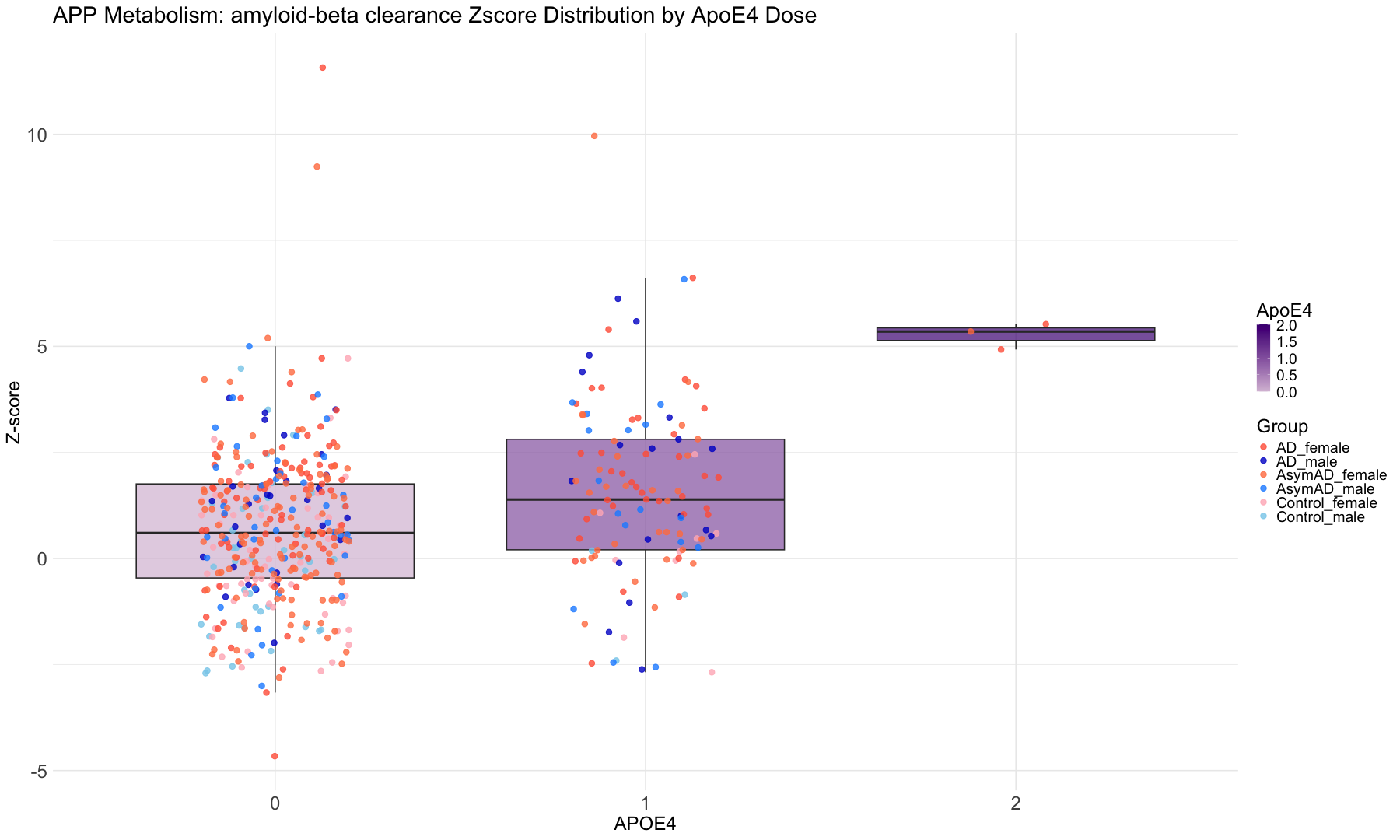
                        "ApoE4.Dose" = "APOE4",
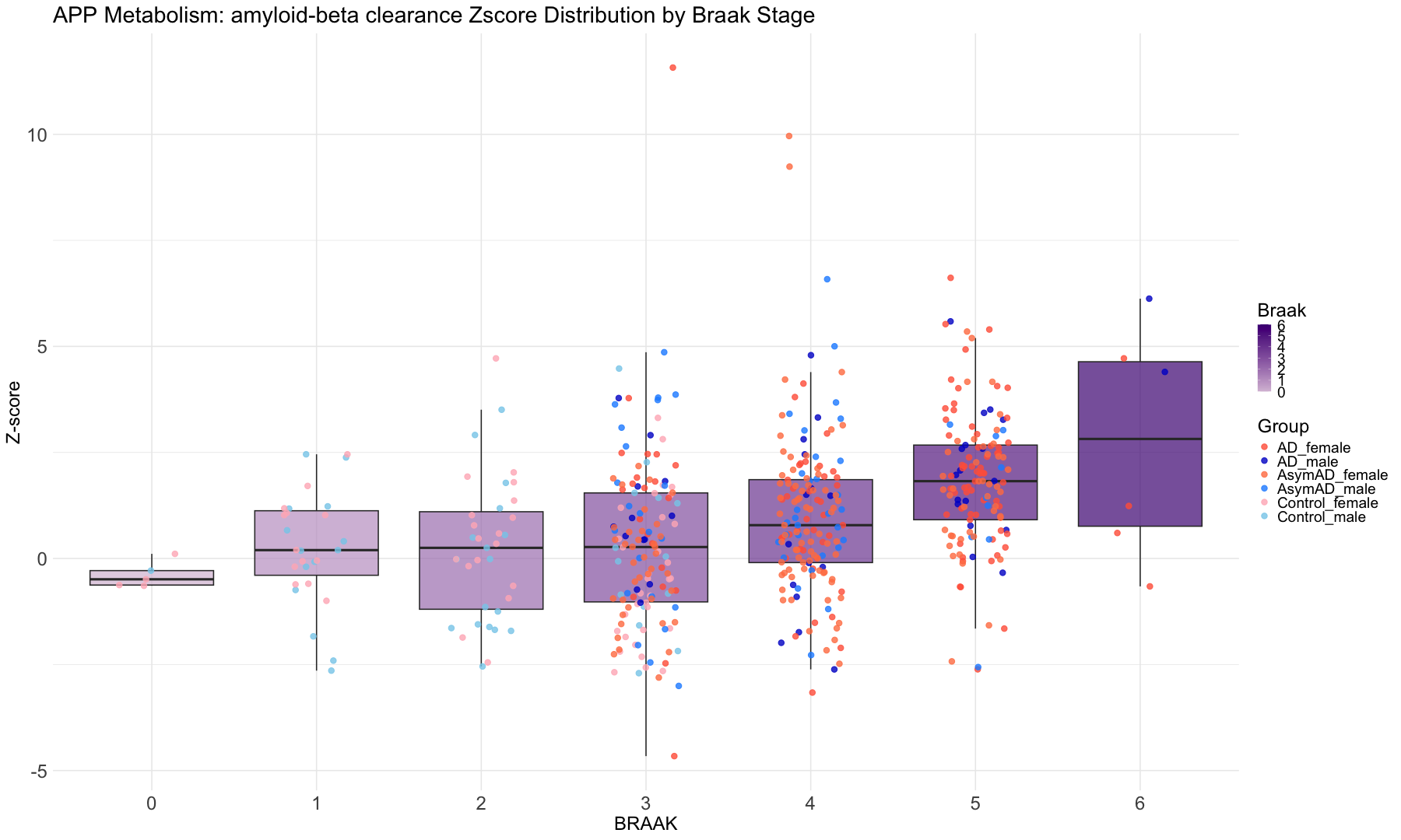
                        "braaksc" = "BRAAK",
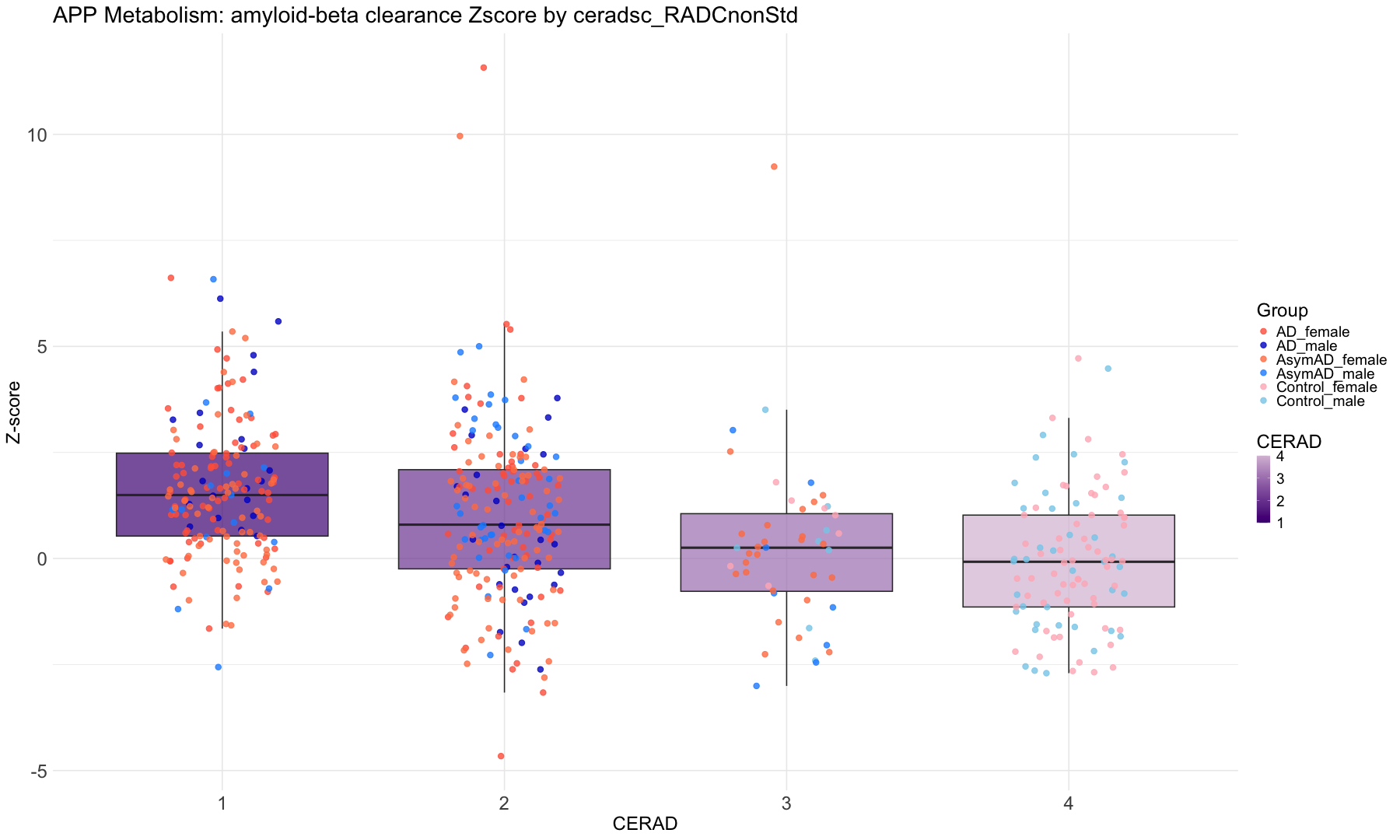
                        "ceradsc_RADCnonStd" = "CERAD",
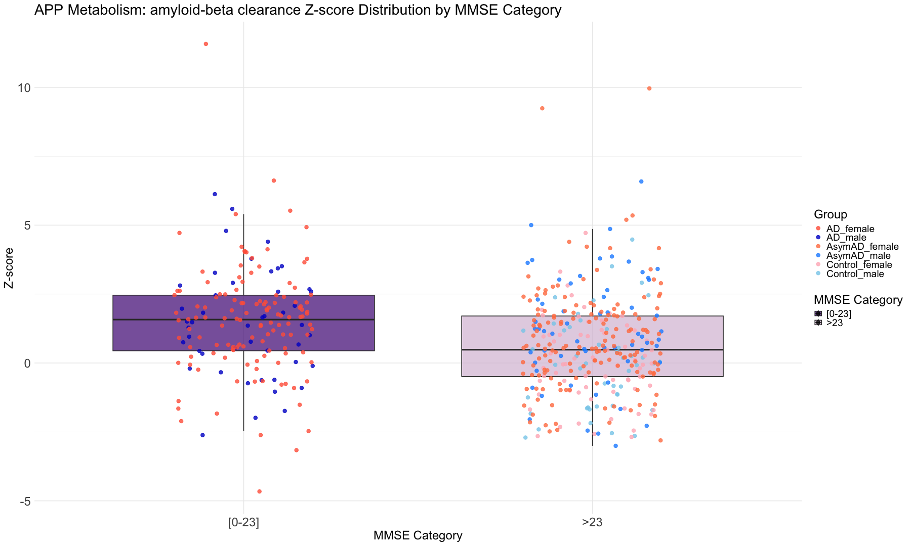
                        "cts_mmse30_lv"= "MMSE"
                        )

# Step 2: Reorder Metadata as factor with desired order
data$Metadata <- factor(data$Metadata, levels = c("APOE4", "CERAD", "BRAAK", "MMSE"))


# Step 3: Identify Biodomain_Subdomain values that appear in more than one Metadata
#common_subdomains <- data %>%
  #group_by(Biodomain_Subdomain) %>%
  #summarise(n_metadata = n_distinct(Metadata)) %>%
  #filter(n_metadata > 1) %>%
  #pull(Biodomain_Subdomain)

# Step 4: Add a flag to the original data
#data <- data %>%
  #mutate(is_common = Biodomain_Subdomain %in% common_subdomains)


# Step 5:Order data by Biodomain and Biodomain_Subdomain
data <- data %>%
  arrange(Biodomain, Biodomain_Subdomain)

# Step 6:Create factor with correct order
data$Biodomain_Subdomain <- factor(data$Biodomain_Subdomain, levels = unique(data$Biodomain_Subdomain))

# Step 7:Determine y positions for rectangles
biodomain_bounds <- data %>%
  distinct(Biodomain, Biodomain_Subdomain) %>%
  group_by(Biodomain) %>%
  summarise(
    ymin = min(as.numeric(Biodomain_Subdomain)) - 0.5,
    ymax = max(as.numeric(Biodomain_Subdomain)) + 0.5
  )


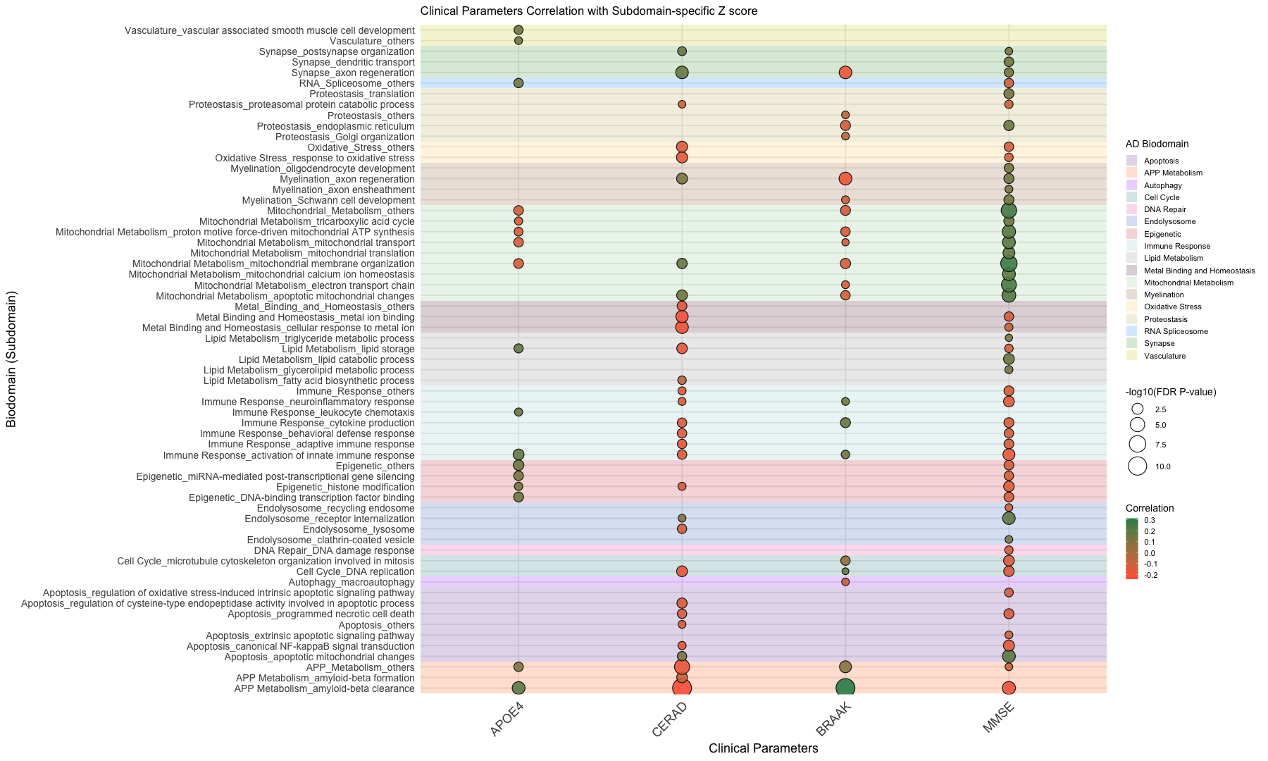
# Plot
ggplot(data, aes(x = Metadata, y = Biodomain_Subdomain)) +

  # Draw background boxes per Biodomain group
  geom_rect(data = biodomain_bounds,
            aes(xmin = -Inf, xmax = Inf, ymin = ymin, ymax = ymax, fill = Biodomain),
            inherit.aes = FALSE, alpha = 0.20) +
  scale_fill_manual(values = custom_colors, name = "AD Biodomain") +

  # Reset fill scale for correlation bubble color
  new_scale_fill() +

  # Bubble plot layer
  geom_point(aes(fill = correlation, size = nl10_FDR_p_value),
             shape = 21, color = "black", alpha = 0.9) +
  scale_fill_gradient(low = "tomato", high = "seagreen", name = "Correlation") +
  scale_size(range = c(4, 12), name = "-log10(FDR P-value)") +

      # Box outline overlay for common points
    #geom_point(
        #data = subset(data, is_common),
        #aes(x = Metadata, y = Biodomain_Subdomain),
        #shape = 0,  # square outline
        #stroke = 1.5,  # Line thickness
        #color = "black",  # Outline color
        #fill = NA,      # Transparent fill to create a "box" effect
        #size = 8        # Match or slightly larger than base point size
    #) +

  # Labels and theme
  labs(
    title = "Clinical Parameters Correlation with Subdomain-specific Z score",
    x = "Clinical Parameters",
    y = "Biodomain (Subdomain)"
  ) +
  theme_minimal(base_size = 18) +
  theme(
    text = element_text(size = 14),
    axis.text.x = element_text(size = 18, hjust = 1, angle = 45),
    axis.text.y = element_text(size = 14),
    axis.title = element_text(size = 18),
    strip.text = element_text(size = 24)
  )

#write.table(data, "data_unique.txt", sep = "\t", quote = FALSE, row.names = FALSE)

Clinical Parameter's Correlation with the Subdomain-specific Zscore (TMT Proteomics) for the Samples from ROSMAP Cohort