############################################################################################################################################################################
## Count the number of gene identified in each subdomain
# Function to process each file
process_subdomain_file <- function(file_path, zscore_data) {
# Read the subdomain subdomain file
subdomain_data <- read.delim(file_path, header = TRUE, sep = "\t")
# Merge with zscore_data
merged_data <- merge(subdomain_data, zscore_data, by.x = "symbol", by.y = "Protein_name", all.x = TRUE)
# Identify columns ending with "_Zscore"
zscore_columns <- grep("_Zscore$", names(merged_data), value = TRUE)
# Calculate the number of non-NA values (mapped genes) for each sample
gene_counts <- apply(merged_data[, zscore_columns], 2, function(z_scores) {
return(sum(!is.na(z_scores)))
})
# Remove "_Zscore" suffix from the Sample_ID names
sample_ids <- sub("_Zscore$", "", zscore_columns)
# Create a new data frame with "Sample_ID" and the number of mapped genes
unique_id <- unique(subdomain_data$unique_id)[1]
colname <- paste0(unique_id, "_gene_count")
gene_count_df <- data.frame(Sample_ID = sample_ids)
gene_count_df[[colname]] <- gene_counts
return(gene_count_df)
}
# Path to the directory containing hsa*.txt files
dir_path <- "/Users/poddea/Desktop/ROSMAP_data_100623/TMT_proteomics/Round2/Subdomain/Subdomain_geneset"
# Read the zscore_AD_female data
# zscore_AD_female <- read.delim("zscore_AD_female.txt", header = TRUE, sep = "\t")
# List all hsa*.txt files in the directory
subdomain_files <- list.files(path = dir_path, pattern = "*.txt$", full.names = TRUE)
# Initialize an empty list to store the results
all_gene_counts <- list()
# Process each subdomain file to count the number of mapped genes
for (file in subdomain_files) {
gene_count_result <- process_subdomain_file(file, zscore_AD_female)
all_gene_counts[[file]] <- gene_count_result
}
# Combine all gene count results into one data frame by merging them on Sample_ID
final_gene_counts_AD_female <- Reduce(function(x, y) merge(x, y, by = "Sample_ID", all = TRUE), all_gene_counts)
# Write the final gene counts to a file
write.table(final_gene_counts_AD_female, "subdomain_gene_count_AD_female_summary.txt", sep = "\t", quote = FALSE, row.names = FALSE)
############################################################################################################################################################################
############################################################################################################################################################################
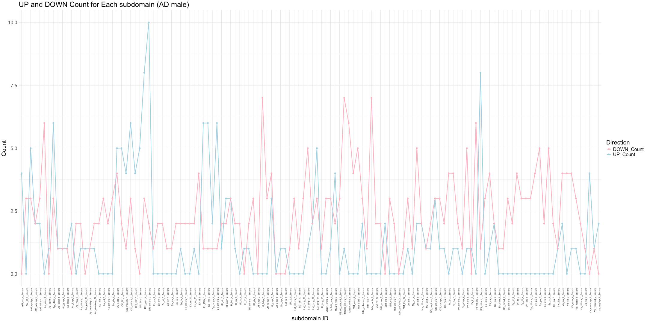
## AD_male
# Function to process each file
process_subdomain_file <- function(file_path, zscore_data) {
# Read the subdomain subdomain file
subdomain_data <- read.delim(file_path, header = TRUE, sep = "\t")
# Merge with zscore_data
merged_data <- merge(subdomain_data, zscore_data, by.x = "symbol", by.y = "Protein_name", all.x = TRUE)
# Identify columns ending with "_Zscore"
zscore_columns <- grep("_Zscore$", names(merged_data), value = TRUE)
# Calculate Stouffer's combined Z-scores for each column
stouffer_zscores <- apply(merged_data[, zscore_columns], 2, function(z_scores) {
# Remove NA values
z_scores <- na.omit(z_scores)
# Calculate the Stouffer's Z-score
stouffer_z <- sum(z_scores) / sqrt(length(z_scores))
return(stouffer_z)
})
# Remove "_Zscore" suffix from the Sample_ID names
sample_ids <- sub("_Zscore$", "", zscore_columns)
# Create a new data frame with "Sample_ID" and the calculated Stouffer's Z-scores
unique_id <- unique(subdomain_data$unique_id)[1]
colname <- paste0(unique_id, "_Zscore")
results_df <- data.frame(Sample_ID = sample_ids)
results_df[[colname]] <- stouffer_zscores
return(results_df)
}
# Path to the directory containing hsa*.txt files
dir_path <- "/Users/poddea/Desktop/ROSMAP_data_100623/TMT_proteomics/Round2/Subdomain/Subdomain_geneset"
# Read the zscore_AD_female data
#zscore_AD_female <- read.delim("zscore_AD_male.txt", header = TRUE, sep = "\t")
# List all hsa*.txt files in the directory
subdomain_files <- list.files(path = dir_path, pattern = "*.txt$", full.names = TRUE)
# Initialize an empty list to store the results
all_results <- list()
# Process each subdomain file
for (file in subdomain_files) {
result <- process_subdomain_file(file, zscore_AD_male)
all_results[[file]] <- result
}
# Combine all results into one data frame by merging them on Sample_ID
final_results_AD_male <- Reduce(function(x, y) merge(x, y, by = "Sample_ID", all = TRUE), all_results)
# Write the final results to a file
write.table(final_results_AD_male, "subdomain_zscore_AD_male_summary.txt", sep = "\t", quote = FALSE, row.names = FALSE)
###########################################################################################################################################################
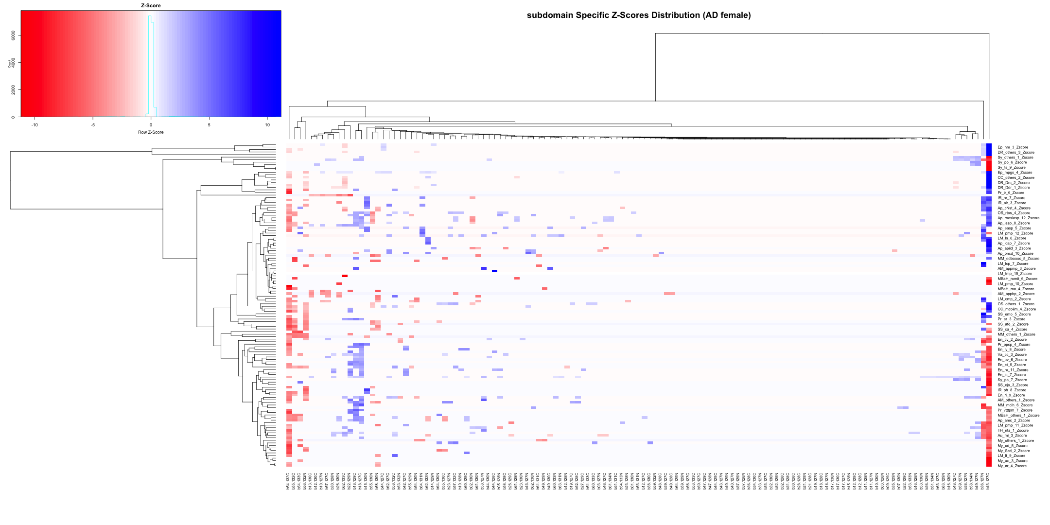
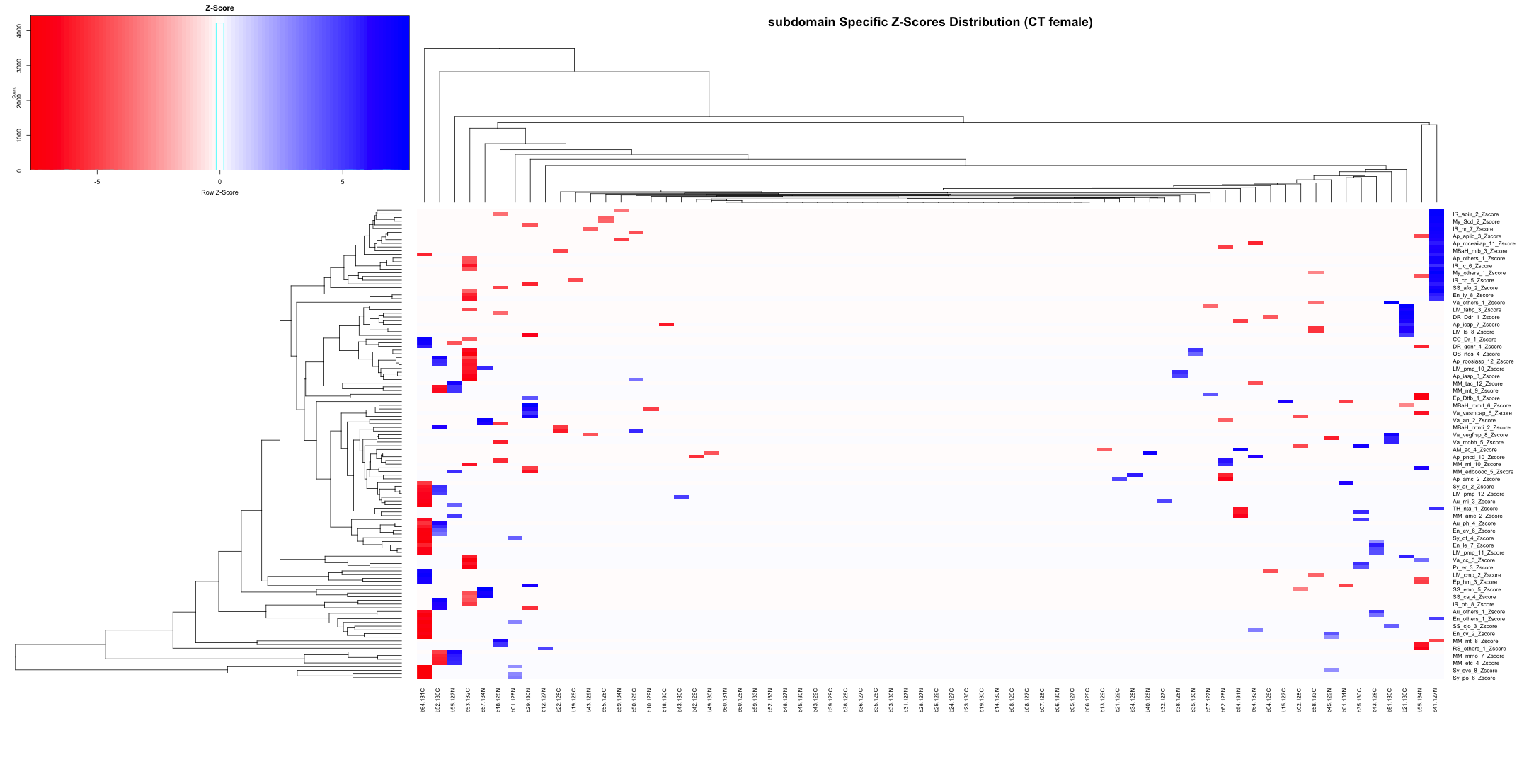
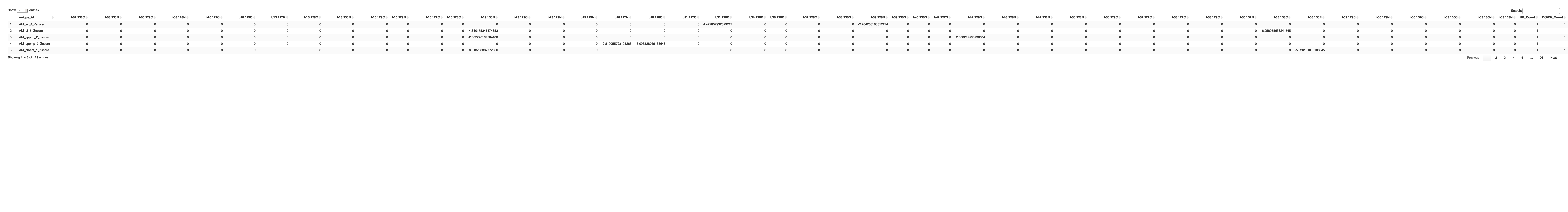
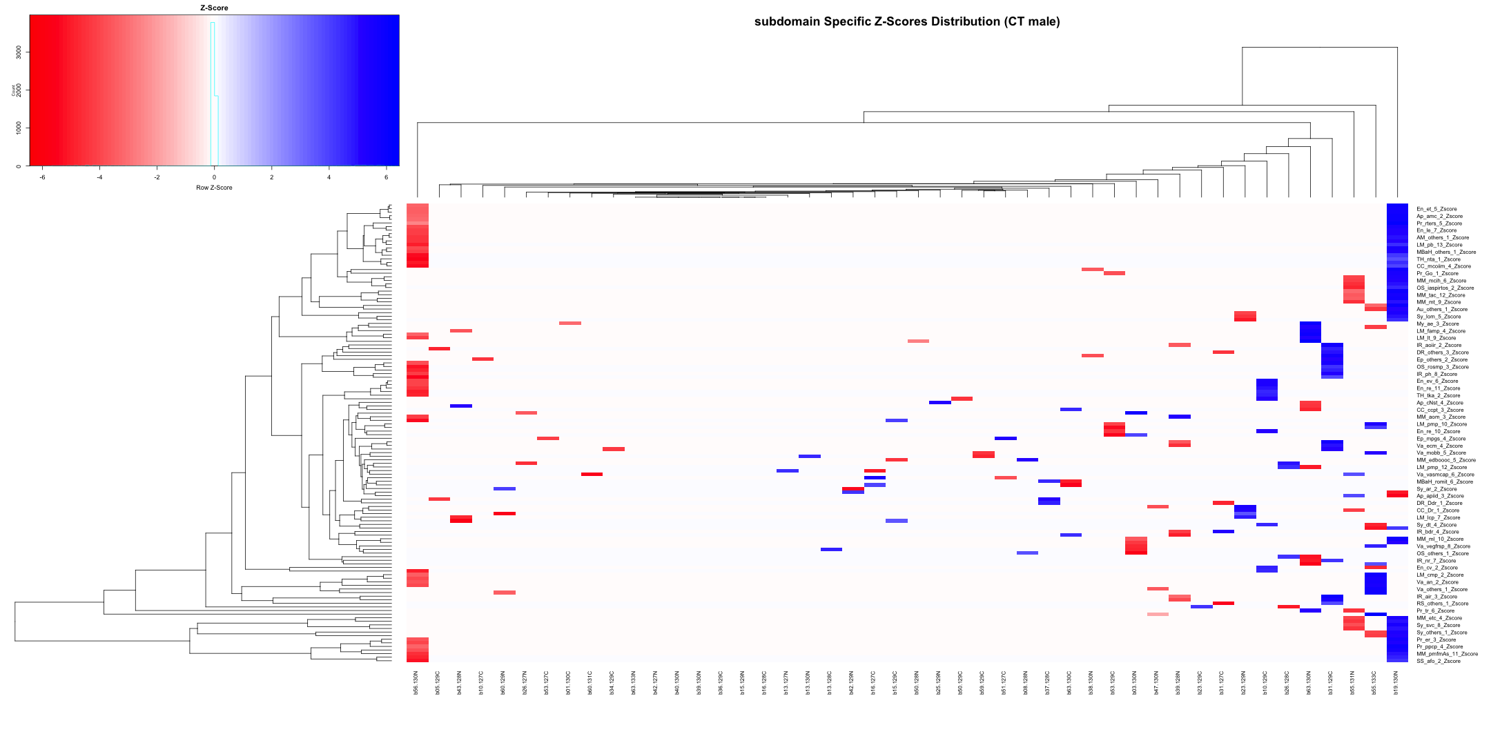
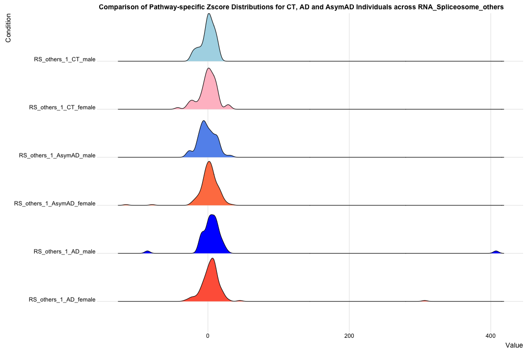
# Transpose the file to count 1st and 99th percentile of the Z score distributions in individual subdomain
final_results_AD_male_t <- as.data.frame(t(final_results_AD_male[,-1]))
colnames(final_results_AD_male_t) <- final_results_AD_male$Sample_ID
# Convert the row names to a new column named "unique_id"
final_results_AD_male_t$unique_id <- rownames(final_results_AD_male_t)
# Reorder the columns so that "unique_id" comes first
final_results_AD_male_t <- final_results_AD_male_t[, c("unique_id", names(final_results_AD_male_t)[-ncol(final_results_AD_male_t)])]
# Reset the row names as they are no longer needed
rownames(final_results_AD_male_t) <- NULL
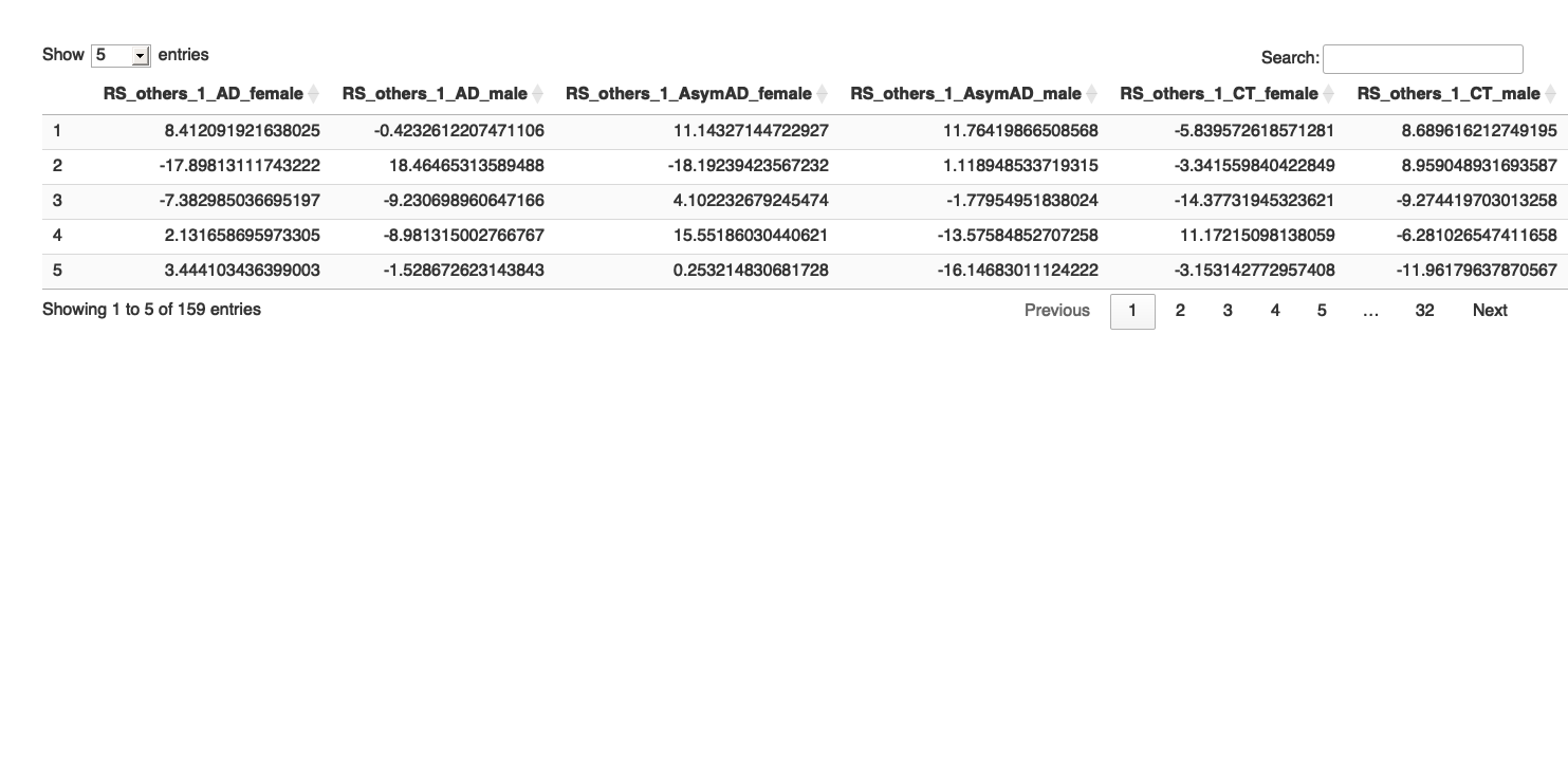
# Print the table using DT
datatable(final_results_AD_male_t, options = list(pageLength = 5, autoWidth = TRUE))