Avijit Podder Date: Aug 12, 2024

library(gplots)

## 
## Attaching package: 'gplots'

## The following object is masked from 'package:stats':
## 
##     lowess

library("ggplot2")

## Warning: package 'ggplot2' was built under R version 4.5.2

library(reshape2)
library(RColorBrewer)
library(dplyr)

## 
## Attaching package: 'dplyr'

## The following objects are masked from 'package:stats':
## 
##     filter, lag

## The following objects are masked from 'package:base':
## 
##     intersect, setdiff, setequal, union

library(viridis)

## Loading required package: viridisLite

library(ggrepel)
library(corrplot)

## corrplot 0.95 loaded

library(plotly)

## 
## Attaching package: 'plotly'

## The following object is masked from 'package:ggplot2':
## 
##     last_plot

## The following object is masked from 'package:stats':
## 
##     filter

## The following object is masked from 'package:graphics':
## 
##     layout

# Open pathways comparison file
#data_KEGG <- read.csv("comparative_pathway_results_proteomics_selected_KEGG.csv", sep =",", header = TRUE, stringsAsFactors = FALSE)

#data_KEGG <- read.csv("comparative_pathway_results.csv", sep =",", header = TRUE, stringsAsFactors = FALSE)

data_KEGG <- read.csv("comparative_pathway_results_proteomics_selected_KEGG_050525.csv", sep =",", header = TRUE, stringsAsFactors = FALSE)

dim(data_KEGG)

## [1] 186  11

head(data_KEGG)

##   Sno Pathway_ID                              Pathway_name UP_ratio_AD_female
## 1   1   hsa00010             Glycolysis / Gluconeogenesis           0.0937500
## 2   3   hsa00030                Pentose phosphate pathway           0.0390625
## 3   4   hsa00040 Pentose and glucuronate interconversions           0.0625000
## 4   5   hsa00051          Fructose and mannose metabolism           0.0859375
## 5   6   hsa00052                     Galactose metabolism           0.1093750
## 6   7   hsa00053        Ascorbate and aldarate metabolism           0.0781250
##   UP_ratio_AD_male DOWN_ratio_AD_female DOWN_ratio_AD_male
## 1       0.04255319            0.0390625         0.04255319
## 2       0.10638298            0.0000000         0.04255319
## 3       0.10638298            0.0234375         0.02127660
## 4       0.08510638            0.0234375         0.04255319
## 5       0.10638298            0.0234375         0.02127660
## 6       0.04255319            0.0156250         0.04255319
##   UP_ratio_AsymAD_female UP_ratio_AsymAD_male DOWN_ratio_AsymAD_female
## 1             0.06289308           0.06557377               0.02515723
## 2             0.01886793           0.06557377               0.01886793
## 3             0.02515723           0.04918033               0.01886793
## 4             0.03144654           0.06557377               0.01886793
## 5             0.05031447           0.04918033               0.02515723
## 6             0.01257862           0.01639344               0.02515723
##   DOWN_ratio_AsymAD_male
## 1             0.06557377
## 2             0.04918033
## 3             0.03278689
## 4             0.03278689
## 5             0.00000000
## 6             0.03278689

# Distribution of Gene_ratio over the pathways
#ggplot(data_KEGG, aes(x = Gene_ratio)) +  
  #geom_histogram(binwidth = 0.05, fill = "blue", color = "black", alpha = 0.7) + 
  #geom_text(stat='bin', binwidth=0.05, aes(label=..count..), vjust=-0.5) + 
  #labs(title = "Histogram of Gene Ratio", x = "Gene Ratio", y = "Frequency") + 
  #theme_minimal() +  
  #theme(text = element_text(size = 16))




# Removing the 1st and 2nd columns
#data_KEGG_new <- data_KEGG[, -c(1, 2, 4, 5, 6)]

data_KEGG_new <- data_KEGG[, -c(1, 2)]

head(data_KEGG_new)

##                                Pathway_name UP_ratio_AD_female UP_ratio_AD_male
## 1             Glycolysis / Gluconeogenesis           0.0937500       0.04255319
## 2                Pentose phosphate pathway           0.0390625       0.10638298
## 3 Pentose and glucuronate interconversions           0.0625000       0.10638298
## 4          Fructose and mannose metabolism           0.0859375       0.08510638
## 5                     Galactose metabolism           0.1093750       0.10638298
## 6        Ascorbate and aldarate metabolism           0.0781250       0.04255319
##   DOWN_ratio_AD_female DOWN_ratio_AD_male UP_ratio_AsymAD_female
## 1            0.0390625         0.04255319             0.06289308
## 2            0.0000000         0.04255319             0.01886793
## 3            0.0234375         0.02127660             0.02515723
## 4            0.0234375         0.04255319             0.03144654
## 5            0.0234375         0.02127660             0.05031447
## 6            0.0156250         0.04255319             0.01257862
##   UP_ratio_AsymAD_male DOWN_ratio_AsymAD_female DOWN_ratio_AsymAD_male
## 1           0.06557377               0.02515723             0.06557377
## 2           0.06557377               0.01886793             0.04918033
## 3           0.04918033               0.01886793             0.03278689
## 4           0.06557377               0.01886793             0.03278689
## 5           0.04918033               0.02515723             0.00000000
## 6           0.01639344               0.02515723             0.03278689

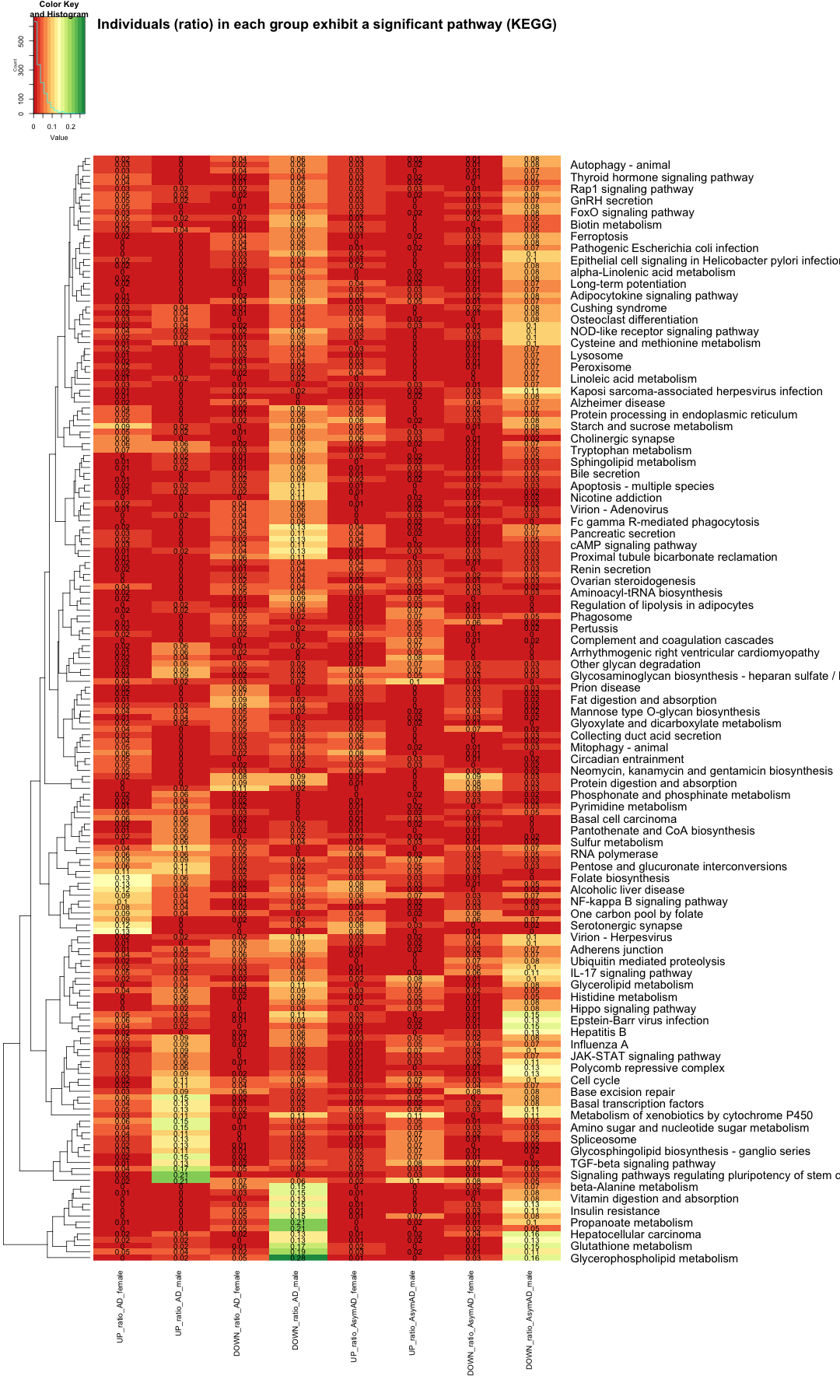
data_matrix_KEGG <- data_KEGG_new[, -1]

# Replace NA values with 0 (or any other specific value)
data_matrix_KEGG[is.na(data_matrix_KEGG)] <- 0

# Set up the color scale using RColorBrewer
color_scale <- colorRampPalette(brewer.pal(9, "RdYlGn"))
color_scale <- colorRampPalette(brewer.pal(9, "RdYlGn"))
color_scale1 <- colorRampPalette(c("white", "lightblue", "blue", "darkblue"))
color_scale2 <- colorRampPalette(brewer.pal(9, "RdGy"))
color_scale3 <- colorRampPalette(brewer.pal(9, "Greens"))
color_scale4 <- colorRampPalette(brewer.pal(9, "Blues"))
color_scale5 <- colorRampPalette(brewer.pal(9, "Purples"))
color_scale6 <- colorRampPalette(brewer.pal(9, "Oranges"))

heatmap.2(
as.matrix(data_matrix_KEGG),
Rowv = TRUE,
Colv = FALSE,
col = color_scale,
scale = "none",  # Scale rows (genes) to Z-scores
trace = "none",  # Turn off row and column annotations
margins = c(15, 30),  # Set margins for row and column labels
key = TRUE,  # Include a color key
keysize = .5,  # Size of the color key
cexCol = 1,  # Set column label size
cexRow = 1.5,  # Set row label size
cellnote=round(data_matrix_KEGG, 2),
notecol="black",
labRow = data_KEGG$Pathway_name,  # Row labels (Pathway name)
dendrogram = "row",  # Show both row and column dendrograms
main="Individuals (ratio) in each group exhibit a significant pathway (KEGG)"
)

# subset the data where the value is equal to or greater than 0.10 in any row 
subset_data_KEGG <- data_KEGG_new %>% filter(UP_ratio_AD_female >= 0.10 | DOWN_ratio_AD_female >= 0.10 | UP_ratio_AD_male >= 0.10 | DOWN_ratio_AD_male >= 0.10 | UP_ratio_AsymAD_female >= 0.10 | DOWN_ratio_AsymAD_female >= 0.10 | UP_ratio_AsymAD_male >= 0.10 | DOWN_ratio_AsymAD_male >= 0.10)

write.table(subset_data_KEGG,"subset_data_KEGG_atleast_10percent_ind.txt",sep="\t",quote=F)


rownames(subset_data_KEGG) <- subset_data_KEGG$Pathway_name

subset_data_KEGG <- subset_data_KEGG[, -1]

# Replace NA values with 0 (or any other specific value)
subset_data_KEGG[is.na(subset_data_KEGG)] <- 0


head(subset_data_KEGG, 3)

##                                           UP_ratio_AD_female UP_ratio_AD_male
## Pentose phosphate pathway                          0.0390625         0.106383
## Pentose and glucuronate interconversions           0.0625000         0.106383
## Galactose metabolism                               0.1093750         0.106383
##                                           DOWN_ratio_AD_female
## Pentose phosphate pathway                            0.0000000
## Pentose and glucuronate interconversions             0.0234375
## Galactose metabolism                                 0.0234375
##                                           DOWN_ratio_AD_male
## Pentose phosphate pathway                         0.04255319
## Pentose and glucuronate interconversions          0.02127660
## Galactose metabolism                              0.02127660
##                                           UP_ratio_AsymAD_female
## Pentose phosphate pathway                             0.01886793
## Pentose and glucuronate interconversions              0.02515723
## Galactose metabolism                                  0.05031447
##                                           UP_ratio_AsymAD_male
## Pentose phosphate pathway                           0.06557377
## Pentose and glucuronate interconversions            0.04918033
## Galactose metabolism                                0.04918033
##                                           DOWN_ratio_AsymAD_female
## Pentose phosphate pathway                               0.01886793
## Pentose and glucuronate interconversions                0.01886793
## Galactose metabolism                                    0.02515723
##                                           DOWN_ratio_AsymAD_male
## Pentose phosphate pathway                             0.04918033
## Pentose and glucuronate interconversions              0.03278689
## Galactose metabolism                                  0.00000000

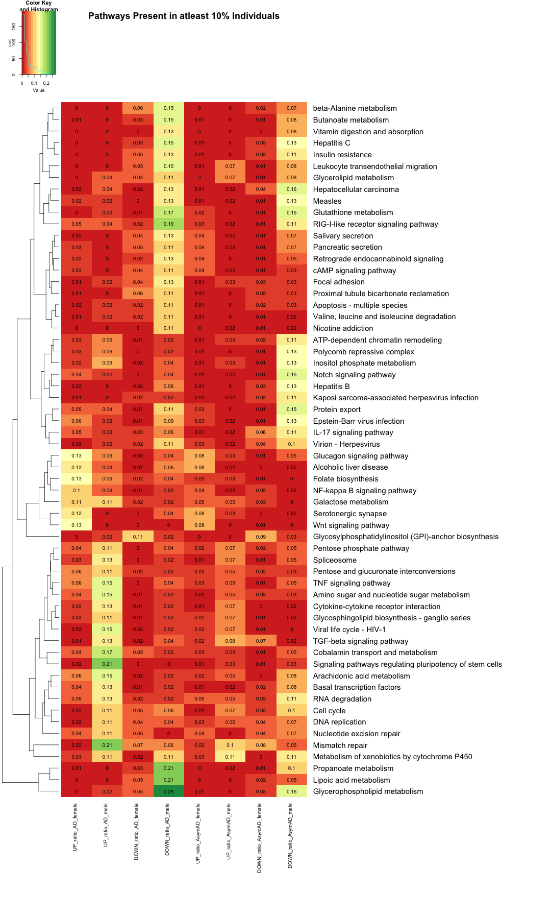
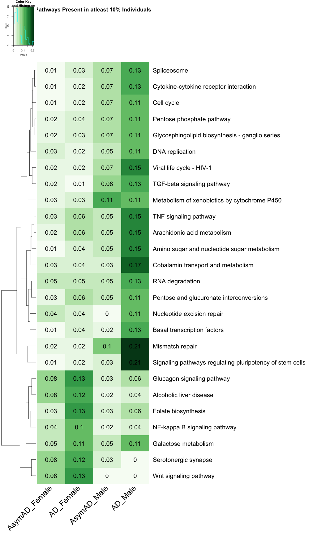
# Create the heatmap with filtered row names
heatmap.2(
     as.matrix(subset_data_KEGG),
     Rowv = TRUE,
     Colv = FALSE,
     col = color_scale,
     scale = "none",
     trace = "none",
     margins = c(20, 40),
     key = TRUE,
     keysize = .5,
     cexCol = 1,
     cexRow = 1.5,
    cellnote=round(subset_data_KEGG, 2),
    notecol="black",
    dendrogram = "row",
    main = "Pathways Present in atleast 10% Individuals"
)

########################################################################################################################################################################################################

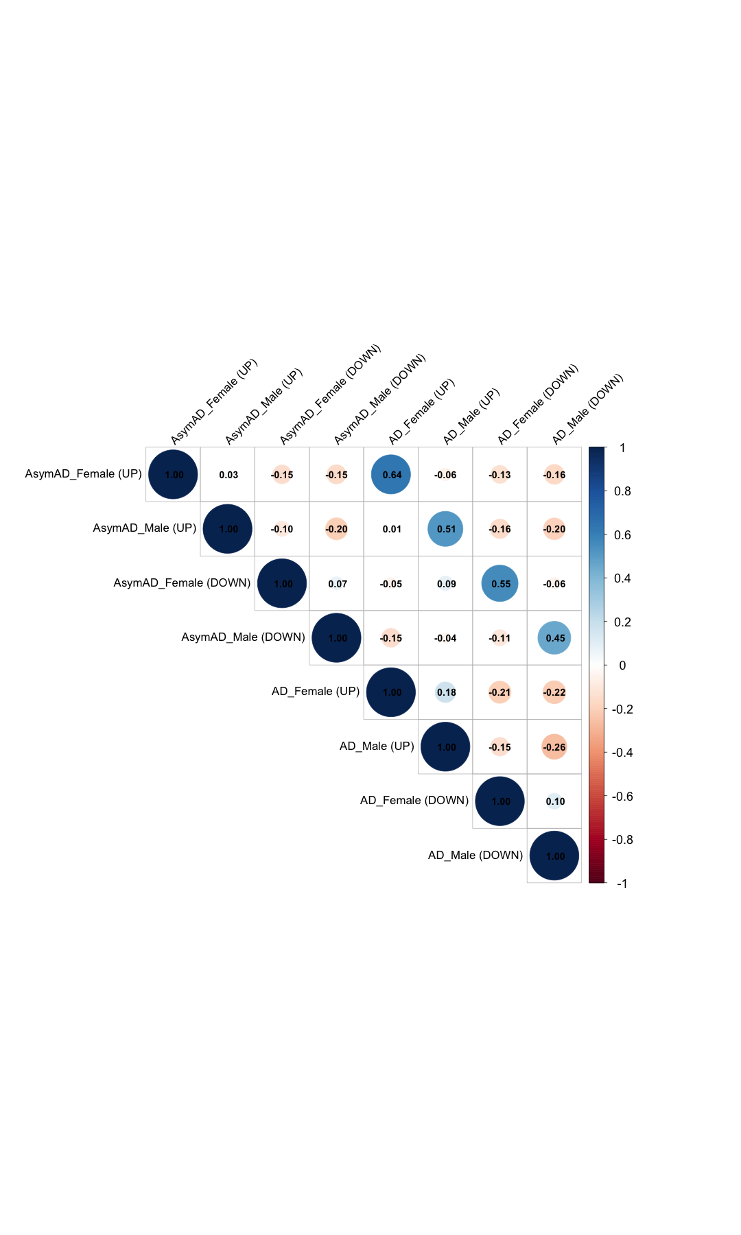
# Filter data_KEGG_new where 'Pathway_name' contains the phrase 'metabolism'
#data_KEGG_new_metabolism <- data_KEGG_new %>%
  #filter(grepl("metabolism", Pathway_name))

#dim(data_KEGG_new_metabolism)

#head(data_KEGG_new_metabolism)

#write.table(data_KEGG_new_metabolism,"data_KEGG_new_metabolism.txt",sep="\t",quote=F)

#data_matrix_KEGG_new_metabolism <- data_KEGG_new_metabolism[, -1]

# Replace NA values with 0 (or any other specific value)
#data_matrix_KEGG_new_metabolism[is.na(data_matrix_KEGG_new_metabolism)] <- 0


#heatmap.2(
     #as.matrix(data_matrix_KEGG_new_metabolism),
     #Rowv = TRUE,
     #Colv = FALSE,
     #col = color_scale,
     #scale = "none",
     #trace = "none",
     #margins = c(20, 40),
     #key = TRUE,
     #keysize = .5,
     #cexCol = 1.5,
     #cexRow = 2,
    #cellnote=round(data_matrix_KEGG_new_metabolism, 2),
    #notecol="black",
    #dendrogram = "row",
    #labRow = data_KEGG_new_metabolism$Pathway_name,
    #main = "Distributions of Metablic Pathways in Each Group"
#)


# Filter data_KEGG_new where 'Pathway_name' contains the phrase 'metabolism'
#data_KEGG_metabolism <- data_KEGG %>%
  #filter(grepl("metabolism", Pathway_name))

# Create the bar plot for Gene_ratio
#ggplot(data_KEGG_metabolism, aes(x = Gene_ratio, y = reorder(Pathway_name, Pathway_name))) +
  #geom_bar(stat = "identity", fill = "steelblue") +
  #labs(title = "Bar Plot of Gene_ratio",
       #x = "Gene ratio",
       #y = "Pathway Name") +
  #theme(axis.text.x = element_text(hjust = 1, size =10),  # Rotate x-axis labels
        #text = element_text(size = 20))  # Adjust text size

########################################################################################################################################################################################################

# Calculate the correlation matrix

library(corrplot)

# 1. Desired column order (AsymAD first, then AD)
column_order <- c(
    "UP_ratio_AsymAD_female", "UP_ratio_AsymAD_male",
    "DOWN_ratio_AsymAD_female", "DOWN_ratio_AsymAD_male",
    "UP_ratio_AD_female", "UP_ratio_AD_male",
    "DOWN_ratio_AD_female", "DOWN_ratio_AD_male"
)

# 2. Reorder the matrix
data_matrix_KEGG <- data_matrix_KEGG[, column_order]

# 3. Create custom labels
col_labels <- c(
    "AsymAD_Female (UP)",
    "AsymAD_Male (UP)",
    "AsymAD_Female (DOWN)",
    "AsymAD_Male (DOWN)",
    "AD_Female (UP)",
    "AD_Male (UP)",
    "AD_Female (DOWN)",
    "AD_Male (DOWN)"
)

# 4. Compute correlation matrix
correlation_matrix <- cor(data_matrix_KEGG, use = "complete.obs")

# 5. Rename both row and column names for corrplot
colnames(correlation_matrix) <- col_labels
rownames(correlation_matrix) <- col_labels

# 6. Draw the correlation plot
corrplot(
    correlation_matrix,
    method = "circle",
    type = "upper",
    tl.col = "black",
    tl.cex = 1.4,          # Axis label font size
    number.cex = 1.2,      # Correlation number font size
    addCoef.col = "black",
    diag = TRUE,
    tl.srt = 45,           # Rotate labels
    cl.cex = 1.5           # ⬅️ Increase color bar font size
)

########################################################################################################################################################################################################
# UP and DOWN Pathway Separate ploting 

# Removing the 1st and 2nd columns
#data_KEGG_new_UP <- data_KEGG[, -c(1, 2, 4, 5, 6, 8, 10, 12, 14)]

data_KEGG_new_UP <- data_KEGG[, -c(1, 2, 6, 7, 10, 11)]

head(data_KEGG_new_UP)

##                                Pathway_name UP_ratio_AD_female UP_ratio_AD_male
## 1             Glycolysis / Gluconeogenesis           0.0937500       0.04255319
## 2                Pentose phosphate pathway           0.0390625       0.10638298
## 3 Pentose and glucuronate interconversions           0.0625000       0.10638298
## 4          Fructose and mannose metabolism           0.0859375       0.08510638
## 5                     Galactose metabolism           0.1093750       0.10638298
## 6        Ascorbate and aldarate metabolism           0.0781250       0.04255319
##   UP_ratio_AsymAD_female UP_ratio_AsymAD_male
## 1             0.06289308           0.06557377
## 2             0.01886793           0.06557377
## 3             0.02515723           0.04918033
## 4             0.03144654           0.06557377
## 5             0.05031447           0.04918033
## 6             0.01257862           0.01639344

#data_KEGG_new_DOWN <- data_KEGG[, -c(1, 2, 4, 5, 6, 7, 9, 11, 13)]

data_KEGG_new_DOWN <- data_KEGG[, -c(1, 2, 4, 5, 8, 9)]

head(data_KEGG_new_DOWN)

##                                Pathway_name DOWN_ratio_AD_female
## 1             Glycolysis / Gluconeogenesis             0.0390625
## 2                Pentose phosphate pathway             0.0000000
## 3 Pentose and glucuronate interconversions             0.0234375
## 4          Fructose and mannose metabolism             0.0234375
## 5                     Galactose metabolism             0.0234375
## 6        Ascorbate and aldarate metabolism             0.0156250
##   DOWN_ratio_AD_male DOWN_ratio_AsymAD_female DOWN_ratio_AsymAD_male
## 1         0.04255319               0.02515723             0.06557377
## 2         0.04255319               0.01886793             0.04918033
## 3         0.02127660               0.01886793             0.03278689
## 4         0.04255319               0.01886793             0.03278689
## 5         0.02127660               0.02515723             0.00000000
## 6         0.04255319               0.02515723             0.03278689

data_matrix_KEGG_UP <- data_KEGG_new_UP[, -1]
data_matrix_KEGG_DOWN <- data_KEGG_new_DOWN[, -1]

# Reorder the columns
data_matrix_KEGG_UP <- data_matrix_KEGG_UP[, c(
  "UP_ratio_AsymAD_female",
  "UP_ratio_AD_female",
  "UP_ratio_AsymAD_male",
  "UP_ratio_AD_male"
)]

data_matrix_KEGG_DOWN <- data_matrix_KEGG_DOWN[, c(
  "DOWN_ratio_AsymAD_female",
  "DOWN_ratio_AD_female",
  "DOWN_ratio_AsymAD_male",
  "DOWN_ratio_AD_male"

)]


# Assign custom column names
colnames(data_matrix_KEGG_UP) <- c("AD_Female", "AsymAD_Female", "AD_Male", "AsymAD_Male")
colnames(data_matrix_KEGG_DOWN) <- c("AD_Female", "AsymAD_Female", "AD_Male", "AsymAD_Male")


# Replace NA values with 0 (or any other specific value)
data_matrix_KEGG_UP[is.na(data_matrix_KEGG_UP)] <- 0
data_matrix_KEGG_DOWN[is.na(data_matrix_KEGG_DOWN)] <- 0

# Set up the color scale using RColorBrewer
color_scale <- colorRampPalette(brewer.pal(9, "RdYlGn"))


heatmap.2(
as.matrix(data_matrix_KEGG_UP),
Rowv = TRUE,
Colv = FALSE,
col = color_scale3,
scale = "none",  # Scale rows (genes) to Z-scores
trace = "none",  # Turn off row and column annotations
margins = c(20, 40),  # Set margins for row and column labels
key = TRUE,  # Include a color key
keysize = .5,  # Size of the color key
cexCol = 1.5,  # Set column label size
cexRow = 1.5,  # Set row label size
cellnote=round(data_matrix_KEGG_UP, 2),
notecol="black",
labRow = data_KEGG$Pathway_name,  # Row labels (Pathway name)
dendrogram = "row",  # Show both row and column dendrograms
main="Individuals (ratio) in each group exhibit a significant pathway (KEGG)"
)

heatmap.2(
as.matrix(data_matrix_KEGG_DOWN),
Rowv = TRUE,
Colv = FALSE,
col = color_scale6,
scale = "none",  # Scale rows (genes) to Z-scores
trace = "none",  # Turn off row and column annotations
margins = c(20, 40),  # Set margins for row and column labels
key = TRUE,  # Include a color key
keysize = .5,  # Size of the color key
cexCol = 1.5,  # Set column label size
cexRow = 1.5,  # Set row label size
cellnote=round(data_matrix_KEGG_DOWN, 2),
notecol="black",
labRow = data_KEGG$Pathway_name,  # Row labels (Pathway name)
dendrogram = "row",  # Show both row and column dendrograms
main="Individuals (ratio) in each group exhibit a significant pathway (KEGG)"
)

##################################################################################################################################################


subset_data_KEGG_UP <- data_KEGG_new_UP %>% filter(UP_ratio_AD_female >= 0.10 | UP_ratio_AD_male >= 0.10 | UP_ratio_AsymAD_female >= 0.10 | UP_ratio_AsymAD_male >= 0.10)

subset_data_KEGG_DOWN <- data_KEGG_new_DOWN %>% filter(DOWN_ratio_AD_female >= 0.10 | DOWN_ratio_AD_male >= 0.10 | DOWN_ratio_AsymAD_female >= 0.10 | DOWN_ratio_AsymAD_male >= 0.10)


rownames(subset_data_KEGG_UP) <- subset_data_KEGG_UP$Pathway_name
rownames(subset_data_KEGG_DOWN) <- subset_data_KEGG_DOWN$Pathway_name


subset_data_KEGG_UP <- subset_data_KEGG_UP[, -1]
subset_data_KEGG_DOWN <- subset_data_KEGG_DOWN[, -1]


# Replace NA values with 0 (or any other specific value)
subset_data_KEGG_UP[is.na(subset_data_KEGG_UP)] <- 0
subset_data_KEGG_DOWN[is.na(subset_data_KEGG_DOWN)] <- 0


head(subset_data_KEGG_UP, 3)

##                                           UP_ratio_AD_female UP_ratio_AD_male
## Pentose phosphate pathway                          0.0390625         0.106383
## Pentose and glucuronate interconversions           0.0625000         0.106383
## Galactose metabolism                               0.1093750         0.106383
##                                           UP_ratio_AsymAD_female
## Pentose phosphate pathway                             0.01886793
## Pentose and glucuronate interconversions              0.02515723
## Galactose metabolism                                  0.05031447
##                                           UP_ratio_AsymAD_male
## Pentose phosphate pathway                           0.06557377
## Pentose and glucuronate interconversions            0.04918033
## Galactose metabolism                                0.04918033

head(subset_data_KEGG_DOWN, 3)

##                                             DOWN_ratio_AD_female
## Valine, leucine and isoleucine degradation             0.0234375
## beta-Alanine metabolism                                0.0625000
## Glutathione metabolism                                 0.0078125
##                                             DOWN_ratio_AD_male
## Valine, leucine and isoleucine degradation           0.1063830
## beta-Alanine metabolism                              0.1489362
## Glutathione metabolism                               0.1702128
##                                             DOWN_ratio_AsymAD_female
## Valine, leucine and isoleucine degradation               0.006289308
## beta-Alanine metabolism                                  0.018867925
## Glutathione metabolism                                   0.012578616
##                                             DOWN_ratio_AsymAD_male
## Valine, leucine and isoleucine degradation              0.01639344
## beta-Alanine metabolism                                 0.06557377
## Glutathione metabolism                                  0.14754098

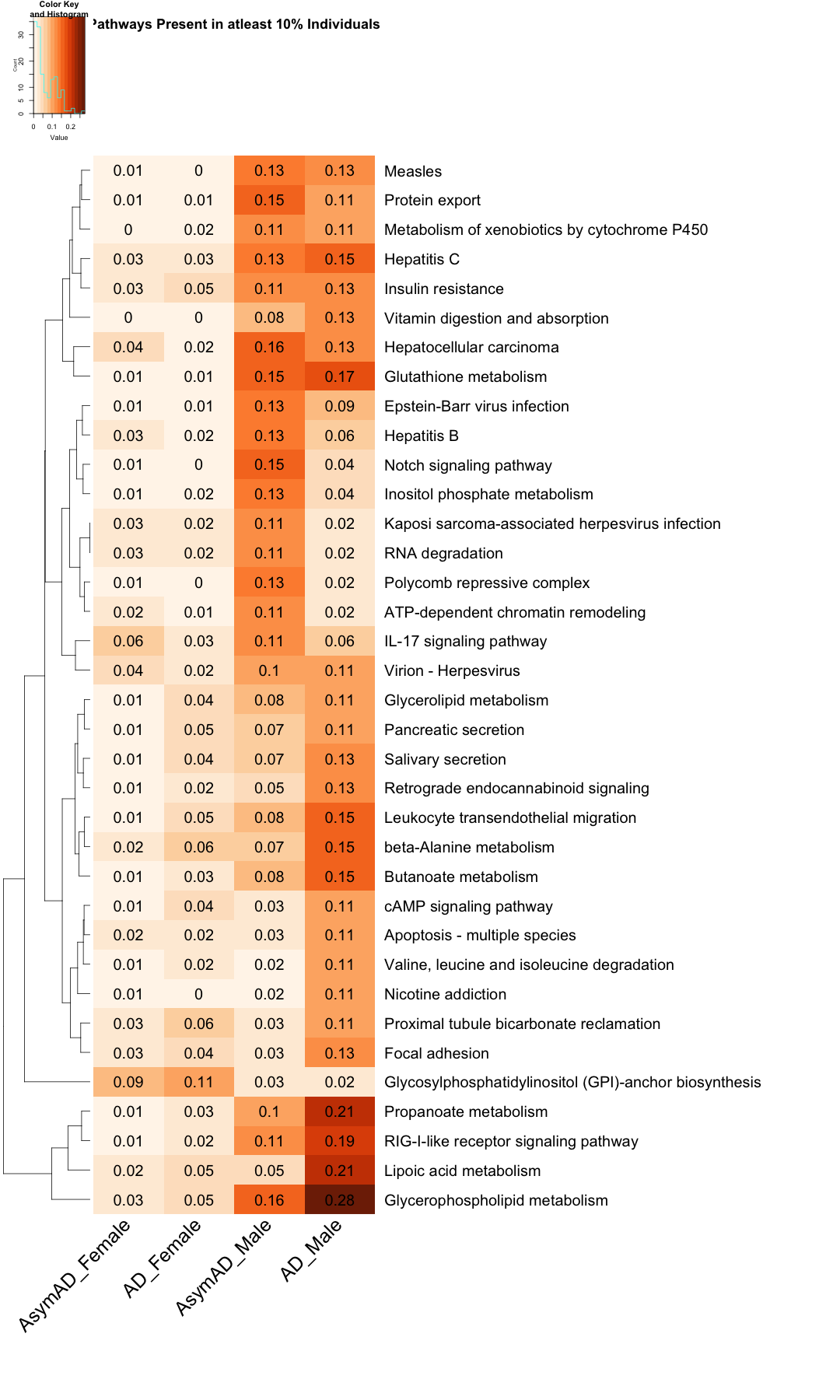
# Reorder the columns
subset_data_KEGG_UP <- subset_data_KEGG_UP[, c(
  "UP_ratio_AsymAD_female",
  "UP_ratio_AD_female",
  "UP_ratio_AsymAD_male",
  "UP_ratio_AD_male"
)]

subset_data_KEGG_DOWN <- subset_data_KEGG_DOWN[, c(
  "DOWN_ratio_AsymAD_female",
  "DOWN_ratio_AD_female",
  "DOWN_ratio_AsymAD_male",
  "DOWN_ratio_AD_male"
)]


# Assign custom column names
colnames(subset_data_KEGG_UP) <- c("AsymAD_Female", "AD_Female",  "AsymAD_Male", "AD_Male")
colnames(subset_data_KEGG_DOWN) <- c("AsymAD_Female", "AD_Female",  "AsymAD_Male", "AD_Male")


# Create the heatmap with filtered row names
UP <- heatmap.2(
     as.matrix(subset_data_KEGG_UP),
     Rowv = TRUE,
     Colv = FALSE,
     col = color_scale3,
     scale = "none",
     trace = "none",
     margins = c(20, 50),
     key = TRUE,
     keysize = .50,
     cexCol = 2.5,
     srtCol = 45,
     cexRow = 2,
    cellnote=round(subset_data_KEGG_UP, 2),
    notecex=2,
    notecol="black",
    dendrogram = "row",
    main = "Pathways Present in atleast 10% Individuals"
)

# Create the heatmap with filtered row names
DOWN <- heatmap.2(
     as.matrix(subset_data_KEGG_DOWN),
     Rowv = TRUE,
     Colv = FALSE,
     col = color_scale6,
     scale = "none",
     trace = "none",
     margins = c(20, 50),
     key = TRUE,
     keysize = .50,
     cexCol = 2.5,
     srtCol = 45,
     cexRow = 2,
    cellnote=round(subset_data_KEGG_DOWN, 2),
    notecex=2,
    notecol="black",
    dendrogram = "row",
    main = "Pathways Present in atleast 10% Individuals"
)

########################################################################################################################################################################################################

# Define a custom color palette with distinct colors for each biodomain (different type of Biodomain - color define by Greg Carry)
#custom_colors <- c("Apoptosis" = "#673399", "APP Metabolism" = "#fe6500", "Autophagy" = "#9931fd", "Cell Cycle" = "#18857f", "DNA Repair" = "#f451ad", "Endolysosome" = "#3466cc", "Epigenetic" = "#cb3233", #"Immune Response" = "#9ccdcc", "Lipid Metabolism" = "#989898", "Metal Binding and Homeostasis" = "#4b0d20", "Mitochondrial Metabolism" = "#97cb98", "Myelination" = "#996735", "Oxidative Stress" = "#ffcd66", #"Proteostasis" = "#c8b269", "RNA Spliceosome" = "#0c9aff", "Structural Stabilization" = "#ff9a9a", "Synapse" = "#329a33", "Tau Homeostasis" = "#cb97cb", "Vasculature" = "#cecd02", "none" = "#7f7f7f")


#  Male vs Female AD
# Open the selected pathways where UP (+) and DOWN (-) pathways are merged together in a single column and the data is separated as a comparison for Male vs Female pathways
#data_KEGG_MvF_AD <- read.csv("Male_Female_comarative_pathway_results_final_111324.csv", sep =",", header = TRUE, stringsAsFactors = FALSE)

data_KEGG_MvF_AD <- read.csv("Male_Female_comarative_pathway_results_final_050525.csv", sep =",", header = TRUE, stringsAsFactors = FALSE)

head(data_KEGG_MvF_AD, 5)

##   Sno Pathway_ID                      Pathway_name_initial
## 1   1   hsa00010             Glycolysis / Gluconeogenesis 
## 2   3   hsa00030                Pentose phosphate pathway 
## 3   4   hsa00040 Pentose and glucuronate interconversions 
## 4   5   hsa00051          Fructose and mannose metabolism 
## 5   6   hsa00052                     Galactose metabolism 
##                                  Pathway_name    Female       Male Direction
## 1             Glycolysis / Gluconeogenesis  + 0.0937500 0.04255319        UP
## 2                Pentose phosphate pathway  + 0.0390625 0.10638298        UP
## 3 Pentose and glucuronate interconversions  + 0.0625000 0.10638298        UP
## 4          Fructose and mannose metabolism  + 0.0859375 0.08510638        UP
## 5                     Galactose metabolism  + 0.1093750 0.10638298        UP
##    Difference
## 1 0.051196809
## 2 0.067320479
## 3 0.043882979
## 4 0.000831117
## 5 0.002992021

# Plot the data as a comparison for Male vs Female pathways

ggplot(data_KEGG_MvF_AD, aes(x = Female, y = Male, size = Difference)) +
  geom_point(aes(size = Gene_ratio), alpha=0.6, stroke = 0) +
    theme_bw() +
    # Conditionally label points where Female or Male values are greater than 0.05
    geom_text_repel(
        aes(label = ifelse((Male > 0.10 & Female < 0.10) | (Female > 0.10 & Male < 0.05) | (Female > 0.05 & Male > 0.05), Pathway_name, "")),
        size = 6, max.overlaps = Inf
    ) +
    #scale_color_manual(values = custom_colors) +
    #labs(color = "Biodomain") +
    # Add x = y line
    geom_abline(slope = 1, intercept = 0, linetype = "dashed", color = "gray", size = 0.5) +
    # Add horizontal and vertical dashed lines
    geom_hline(yintercept = 0.05, linetype = "dashed", color = "gray") +
    geom_hline(yintercept = 0.10, linetype = "dashed", color = "red") +
    geom_vline(xintercept = 0.05, linetype = "dashed", color = "gray") +
    geom_vline(xintercept = 0.10, linetype = "dashed", color = "red") +
    labs(title = "Pathways Comparisons for Male_AD vs Female_AD ", x = "Female (% of subjects)", y = "Male (% of subjects)") +
    theme(
    text = element_text(size = 30),
    legend.position = "right",
    axis.text = element_text(size = 30),
    axis.title = element_text(size = 30)
  )

## Warning: Using `size` aesthetic for lines was deprecated in ggplot2 3.4.0.
## ℹ Please use `linewidth` instead.
## This warning is displayed once every 8 hours.
## Call `lifecycle::last_lifecycle_warnings()` to see where this warning was
## generated.

## Error in `geom_point()`:
## ! Problem while computing aesthetics.
## ℹ Error occurred in the 1st layer.
## Caused by error:
## ! object 'Gene_ratio' not found

########################################################################################################################################################################################################

ggplot(data_KEGG_MvF_AD, aes(x = Female, y = Male, size = Difference)) +
    geom_point(alpha = 0.6, stroke = 0) +  # Increased alpha for better visibility
    theme_bw() +

    # Conditionally label points where |Male - Female| >= 0.05
    geom_text_repel(
        aes(label = ifelse((abs(Female - Male) >= 0.10) | (Female > 0.10) | (Female > 0.07 & Male > 0.07), Pathway_name, "")),
        size = 6,
        max.overlaps = Inf  # Ensure all significant labels are shown
    ) +

   # scale_color_manual(values = custom_colors) +

    #labs(color = "Biodomain") +

    # Add x = y reference line
    geom_abline(slope = 1, intercept = 0, linetype = "dashed", color = "gray", linewidth = 0.5) +

    # Add horizontal and vertical threshold lines
    geom_hline(yintercept = 0.05, linetype = "dashed", color = "gray") +
    geom_hline(yintercept = 0.10, linetype = "dashed", color = "red") +
    geom_vline(xintercept = 0.05, linetype = "dashed", color = "gray") +
    geom_vline(xintercept = 0.10, linetype = "dashed", color = "red") +

    labs(title = "Pathway Comparisons for Female_AD vs Male_AD",
         x = "Female (% of subjects)",
         y = "Male (% of subjects)") +

    theme(
        text = element_text(size = 30),
        legend.position = "right",
        axis.text = element_text(size = 30),
        axis.title = element_text(size = 30)
    )

################################################################################################################################################################################################################################################################################################################################################################################################################


#  AD vs AsymAD 
# Open the selected pathways where the Male and Female percentages are combined together to get AD and AsymAD specific pathways
# Further, UP (+) and DOWN (-) pathways are merged together in a single column and the data is separated as a comparison for AD vs AsymAD pathways
#data_KEGG_ADvAsymAD <- read.csv("AD_AsymAD_comarative_pathway_results_final_111324.csv", sep =",", header = TRUE, stringsAsFactors = FALSE)

data_KEGG_ADvAsymAD <- read.csv("AD_AsymAD_comarative_pathway_results_final_050525.csv", sep =",", header = TRUE, stringsAsFactors = FALSE)

head(data_KEGG_ADvAsymAD, 5)

##   Sno Pathway_ID                      Pathway_name_initial
## 1   1   hsa00010             Glycolysis / Gluconeogenesis 
## 2   3   hsa00030                Pentose phosphate pathway 
## 3   4   hsa00040 Pentose and glucuronate interconversions 
## 4   5   hsa00051          Fructose and mannose metabolism 
## 5   6   hsa00052                     Galactose metabolism 
##                                  Pathway_name        AD     AsymAD Direction
## 1             Glycolysis / Gluconeogenesis  + 0.1363032 0.12846685        UP
## 2                Pentose phosphate pathway  + 0.1454455 0.08444169        UP
## 3 Pentose and glucuronate interconversions  + 0.1688830 0.07433756        UP
## 4          Fructose and mannose metabolism  + 0.1710439 0.09702031        UP
## 5                     Galactose metabolism  + 0.2157580 0.09949479        UP
##    Difference
## 1 0.007836339
## 2 0.061003784
## 3 0.094545418
## 4 0.074023572
## 5 0.116263185

# Plot the data as a comparison for AD vs AsymAD pathways

ggplot(data_KEGG_ADvAsymAD, aes(x = AsymAD, y = AD, size = Difference)) +
  geom_point(aes(size = Gene_ratio), alpha=0.6, stroke = 0) +
    theme_bw() +
    # Conditionally label points where AD or AsymAD values are greater than 0.05
    geom_text_repel(
        aes(label = ifelse((AD > 0.10 & AsymAD < 0.05) | (AsymAD > 0.10 & AD < 0.05) | (AD > 0.10 & AsymAD > 0.10), Pathway_name, "")),
        size = 6, max.overlaps = Inf
    ) +
    #scale_color_manual(values = custom_colors) +
    #labs(color = "Biodomain") +
    # Add x = y line
    geom_abline(slope = 1, intercept = 0, linetype = "dashed", color = "gray", size = 0.5) +
    # Add horizontal and vertical dashed lines
    geom_hline(yintercept = 0.05, linetype = "dashed", color = "gray") +
    geom_hline(yintercept = 0.10, linetype = "dashed", color = "red") +
    geom_vline(xintercept = 0.05, linetype = "dashed", color = "gray") +
    geom_vline(xintercept = 0.10, linetype = "dashed", color = "red") +
    labs(title = "Pathways Comparisons for AD vs AsymAD", x = "AsymAD (% of subjects)", y = "AD (% of subjects)") +
    theme(
    text = element_text(size = 30),
    legend.position = "right",
    axis.text = element_text(size = 30),
    axis.title = element_text(size = 30)
  )

## Error in `geom_point()`:
## ! Problem while computing aesthetics.
## ℹ Error occurred in the 1st layer.
## Caused by error:
## ! object 'Gene_ratio' not found

########################################################################################################################################################################################################

ggplot(data_KEGG_ADvAsymAD, aes(x = AsymAD, y = AD, size = Difference)) +
    geom_point(alpha = 0.6, stroke = 0) +  # Points with transparency
    theme_bw() +

    # Conditionally label points where |AD - AsymAD| >= 0.05
    geom_text_repel(
        aes(label = ifelse((abs(AD - AsymAD) >= 0.10) | (AsymAD > 0.20) | (AD > 0.15 & AsymAD > 0.15), Pathway_name, "")),
        size = 6
    ) +

    #scale_color_manual(values = custom_colors) +
    #labs(color = "Biodomain") +

    # Add x = y reference line
    geom_abline(slope = 1, intercept = 0, linetype = "dashed", color = "gray", size = 0.5) +

    # Add horizontal and vertical threshold lines
    geom_hline(yintercept = 0.05, linetype = "dashed", color = "gray") +
    geom_hline(yintercept = 0.10, linetype = "dashed", color = "red") +
    geom_vline(xintercept = 0.05, linetype = "dashed", color = "gray") +
    geom_vline(xintercept = 0.10, linetype = "dashed", color = "red") +

    # Title and axis labels
    labs(title = "Pathway Comparisons for AD vs AsymAD",
         x = "AsymAD (% of subjects)",
         y = "AD (% of subjects)") +

    # Theme customization
    theme(
        text = element_text(size = 30),
        legend.position = "right",
        axis.text = element_text(size = 30),
        axis.title = element_text(size = 30)
    )

Graph-based Clustering using Pathway Specific Z score Distributions Results (AD male)

Graph-based Clustering using Pathway Specific Z score Distributions Results (AD female)

Individual Pathway Specific Z score Calculation using TMT Proteomic Data from the ROSMAP Cohort (comparative Pathway Profiling - AD-male vs AD-female)