library(jpeg)

# Load the .jpeg image
img <- readJPEG("/Users/poddea/Desktop/ROSMAP_data_100623/Pathway_specific_Zscore.jpg")

# Display the image
plot(1:2, type = "n", xlab = "", ylab = "", axes = FALSE)
rasterImage(img, 1, 1, 2, 2)
library(jpeg) # Load the .jpeg image img <- readJPEG("/Users/poddea/Desktop/ROSMAP_data_100623/Pathway_specific_Zscore.jpg") # Display the image plot(1:2, type = "n", xlab = "", ylab = "", axes = FALSE) rasterImage(img, 1, 1, 2, 2)
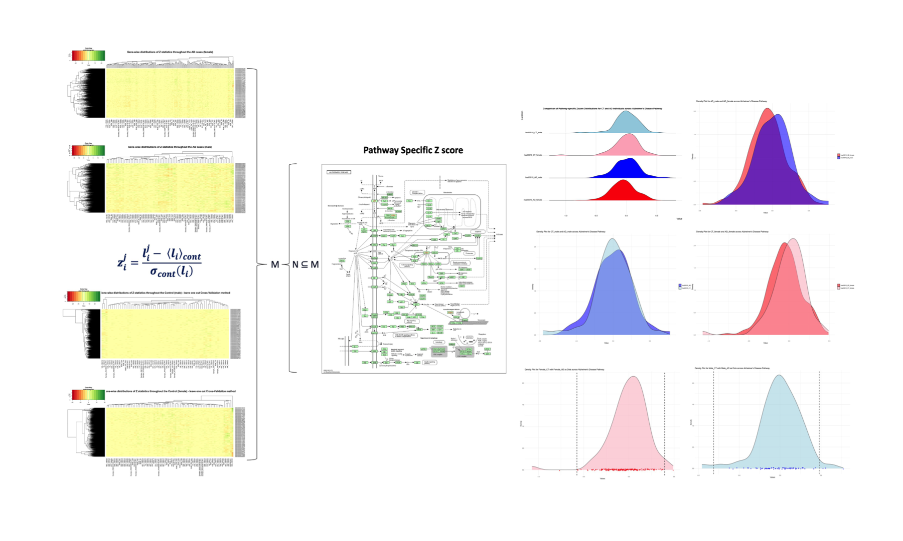
Retrieve human KEGG pathways and genes associated with each pathway:
#Create Individual Pathway Files:
#Open Protein-wise Zscore for CT, AD and AsymAD Individuals (Male and Female Separately):
library(dplyr)
library(tidyr)

## Open individual Zscore distribution files for CT and AD individuals

zscore_CT_male <- read.delim("/Users/poddea/Desktop/ROSMAP_data_100623/TMT_proteomics/Round2/z_stat_result_CT_male.txt", header = TRUE, sep = "\t");

# Ensure column names to` match `IDs` in `zscore_` files
zscore_CT_male <- zscore_CT_male %>% rename_with(~ gsub("X", "", .), starts_with("X"))

dim(zscore_CT_male)
## [1] 7800 47
zscore_CT_female <- read.delim("/Users/poddea/Desktop/ROSMAP_data_100623/TMT_proteomics/Round2/z_stat_result_CT_female.txt", header = TRUE, sep = "\t");

# Ensure column names to` match `IDs` in `zscore_` files
zscore_CT_female <- zscore_CT_female %>% rename_with(~ gsub("X", "", .), starts_with("X"))

dim(zscore_CT_female)
## [1] 7800 69
zscore_AD_male <- read.delim("/Users/poddea/Desktop/ROSMAP_data_100623/TMT_proteomics/Round2/z_stat_result_AD_male.txt", header = TRUE, sep = "\t");

# Ensure column names to` match `IDs` in `zscore_` files
zscore_AD_male <- zscore_AD_male %>% rename_with(~ gsub("X", "", .), starts_with("X"))

dim(zscore_AD_male)
## [1] 7800 48
zscore_AD_female <- read.delim("/Users/poddea/Desktop/ROSMAP_data_100623/TMT_proteomics/Round2/z_stat_result_AD_female.txt", header = TRUE, sep = "\t");

# Ensure column names to` match `IDs` in `zscore_` files
zscore_AD_female <- zscore_AD_female %>% rename_with(~ gsub("X", "", .), starts_with("X"))

dim(zscore_AD_female)
## [1] 7800 128
zscore_AsymAD_male <- read.delim("/Users/poddea/Desktop/ROSMAP_data_100623/TMT_proteomics/Round2/z_stat_result_AsymAD_male.txt", header = TRUE, sep = "\t");

# Ensure column names to` match `IDs` in `zscore_` files
zscore_AsymAD_male <- zscore_AsymAD_male %>% rename_with(~ gsub("X", "", .), starts_with("X"))

dim(zscore_AsymAD_male)
## [1] 7800 62
zscore_AsymAD_female <- read.delim("/Users/poddea/Desktop/ROSMAP_data_100623/TMT_proteomics/Round2/z_stat_result_AsymAD_female.txt", header = TRUE, sep = "\t");

# Ensure column names to` match `IDs` in `zscore_` files
zscore_AsymAD_female <- zscore_AsymAD_female %>% rename_with(~ gsub("X", "", .), starts_with("X"))

dim(zscore_AsymAD_female)
## [1] 7800 160
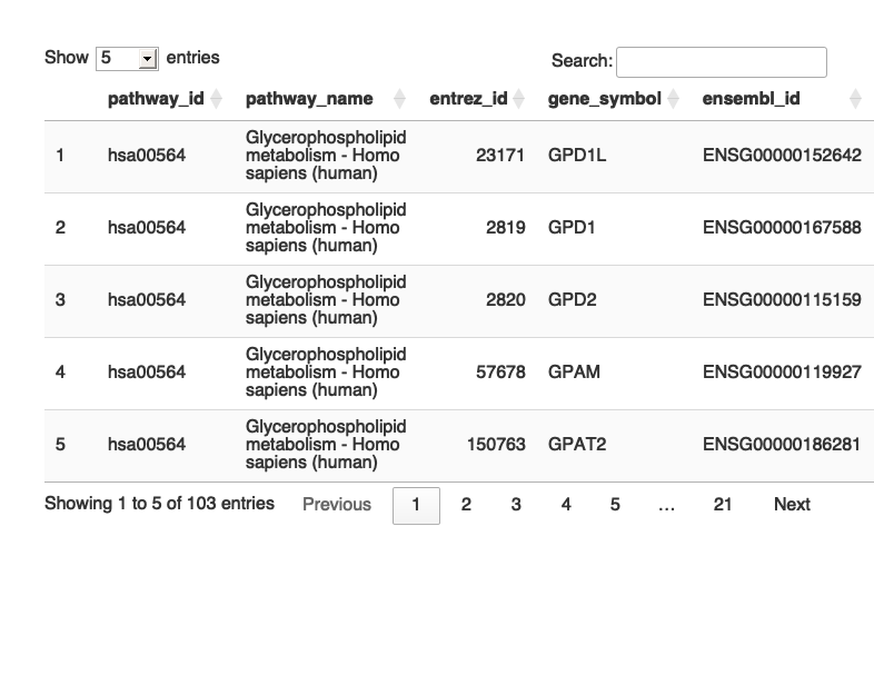
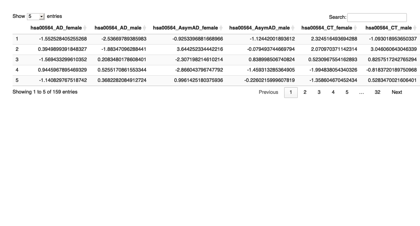
Compare Gene-wise Zscore for CT and AD Individuals across Pathways (Example for Glycerophospholipid metabolism pathway):
library(dplyr)
library(tidyr)
library(DT)

setwd("/Users/poddea/Desktop/ROSMAP_data_100623/TMT_proteomics/Round2/Pathway_sprcific_analysis/kegg_hsa_all")

# Open individual KEGG pathway file
hsa00564 <- read.delim("hsa00564.txt", header = TRUE, sep = "\t");
dim(hsa00564)
## [1] 103 5
#head(hsa00564, 5)

# Print the table using DT
datatable(hsa00564, options = list(pageLength = 5, autoWidth = TRUE))
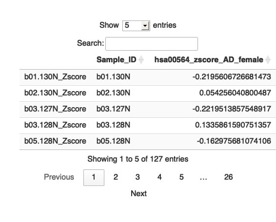
# Merge the data frames
hsa00564_zscore_AD_female <- merge(hsa00564, zscore_AD_female, by.x = "gene_symbol", by.y = "Protein_name", all.x = TRUE)

#head(hsa00564_zscore_AD_female, 2)


# Print the table using DT
datatable(hsa00564_zscore_AD_female, options = list(pageLength = 5, autoWidth = TRUE))

#write.table(hsa04710_zscore_AD_female,"/Users/poddea/Desktop/hsa04710_zscore_AD_female.txt",sep="\t",quote=F, row.name= FALSE)

# Identify columns ending with "_Zscore"
zscore_columns <- grep("_Zscore$", names(hsa00564_zscore_AD_female), value = TRUE)

# Calculate the average for each of these columns
average_zscores <- colMeans(hsa00564_zscore_AD_female[, zscore_columns], na.rm = TRUE)

# Remove "_Zscore" suffix from the Sample_ID names
sample_ids <- sub("_Zscore$", "", zscore_columns)

# Create a new data frame with "Sample_ID" and the calculated averages
Pathway_zscore_AD_female <- data.frame(Sample_ID = sample_ids, hsa00564_zscore_AD_female = average_zscores)

#head(Pathway_zscore_AD_female)

# Print the table using DT
datatable(Pathway_zscore_AD_female, options = list(pageLength = 5, autoWidth = TRUE))
# Write the new data frame to a file
#write.table(Pathway_zscore_AD_female, "/Users/poddea/Desktop/Pathway_zscore_AD_female.txt", sep = "\t", quote = FALSE, row.names = FALSE)
Compare Gene-wise Zscore for CT, AD and AsymAD Individuals across Pathways:
library(ggplot2)
## Warning: package 'ggplot2' was built under R version 4.5.2
library(gplots)
library(RColorBrewer)
library(dplyr)
library(tidyr)
library(DT)

############################################################################################################################################################################
## AD_female

# Function to process each file
process_kegg_file <- function(file_path, zscore_data) {
  # Read the KEGG pathway file
  kegg_data <- read.delim(file_path, header = TRUE, sep = "\t")

  # Merge with zscore_data
  merged_data <- merge(kegg_data, zscore_data, by.x = "gene_symbol", by.y = "Protein_name", all.x = TRUE)

  # Identify columns ending with "_Zscore"
  zscore_columns <- grep("_Zscore$", names(merged_data), value = TRUE)

  # Calculate Stouffer's combined Z-scores for each column
  stouffer_zscores <- apply(merged_data[, zscore_columns], 2, function(z_scores) {
    # Remove NA values
    z_scores <- na.omit(z_scores)

    # Calculate the Stouffer's Z-score
    stouffer_z <- sum(z_scores) / sqrt(length(z_scores))

    return(stouffer_z)
  })

  # Remove "_Zscore" suffix from the Sample_ID names
  sample_ids <- sub("_Zscore$", "", zscore_columns)

  # Create a new data frame with "Sample_ID" and the calculated Stouffer's Z-scores
  pathway_id <- unique(kegg_data$pathway_id)[1]
  colname <- paste0(pathway_id, "_Zscore")
  results_df <- data.frame(Sample_ID = sample_ids)
  results_df[[colname]] <- stouffer_zscores

  return(results_df)
}

# Path to the directory containing hsa*.txt files
dir_path <- "/Users/poddea/Desktop/ROSMAP_data_100623/TMT_proteomics/Round2/Pathway_sprcific_analysis/kegg_hsa_all"

# Read the zscore_AD_female data
#zscore_AD_female <- read.delim("zscore_AD_female.txt", header = TRUE, sep = "\t")

# List all hsa*.txt files in the directory
kegg_files <- list.files(path = dir_path, pattern = "^hsa.*\\.txt$", full.names = TRUE)

# Initialize an empty list to store the results
all_results <- list()

# Process each KEGG file
for (file in kegg_files) {
  result <- process_kegg_file(file, zscore_AD_female)
  all_results[[file]] <- result
}

# Combine all results into one data frame by merging them on Sample_ID
final_results_AD_female <- Reduce(function(x, y) merge(x, y, by = "Sample_ID", all = TRUE), all_results)

# Write the final results to a file
write.table(final_results_AD_female, "Pathway_zscore_AD_female_summary.txt", sep = "\t", quote = FALSE, row.names = FALSE)

###########################################################################################################################################################
# Transpose the file to count 1st and 99th percentile of the Z score distributions in individual pathway
final_results_AD_female_t <- as.data.frame(t(final_results_AD_female[,-1]))

colnames(final_results_AD_female_t) <- final_results_AD_female$Sample_ID

# Convert the row names to a new column named "Pathway_ID"
final_results_AD_female_t$Pathway_ID <- rownames(final_results_AD_female_t)

# Reorder the columns so that "Pathway_ID" comes first
final_results_AD_female_t <- final_results_AD_female_t[, c("Pathway_ID", names(final_results_AD_female_t)[-ncol(final_results_AD_female_t)])]

# Reset the row names as they are no longer needed
rownames(final_results_AD_female_t) <- NULL

# Print the table using DT
datatable(final_results_AD_female_t, options = list(pageLength = 5, autoWidth = TRUE))

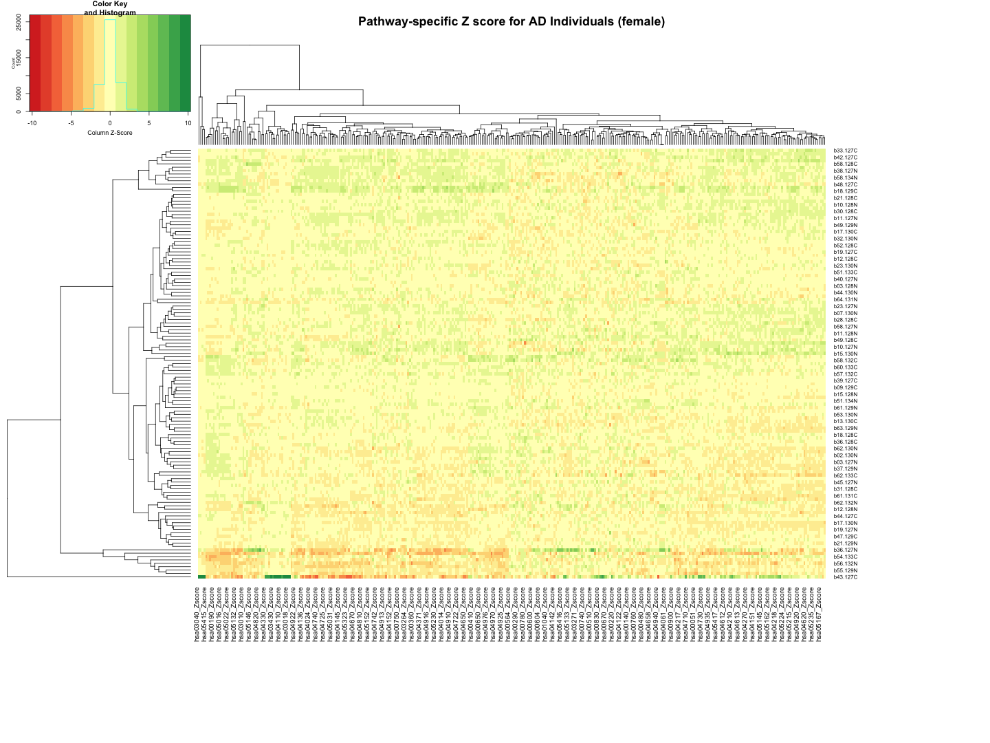
###########################################################################################################################################################
# Plot tha data
# Set rownames to Sample_ID and remove Sample_ID column
rownames(final_results_AD_female) <- final_results_AD_female$Sample_ID

final_results_AD_female <- final_results_AD_female[, -1]

# Remove columns with NA values
final_results_AD_female <- final_results_AD_female[, colSums(is.na(final_results_AD_female)) == 0]


# Set up the color scale using RColorBrewer
color_scale <- colorRampPalette(brewer.pal(9, "RdYlGn"))

# Plot the heatmap using heatmap.2
heatmap.2(
as.matrix(final_results_AD_female),
Rowv = TRUE,
Colv = TRUE,
col = color_scale,
scale = "column",  # Scale rows (genes) to Z-scores
trace = "none",  # Turn off row and column annotations
margins = c(20, 20),  # Set margins for row and column labels
#col = cm.colors(256),  # Set the color map (256 colors)
key = TRUE,  # Include a color key
keysize = 1,  # Size of the color key
cexCol = 1,  # Set column label size
cexRow = 0.8,  # Set row label size
dendrogram = "both",  # Show both row and column dendrograms
main="Pathway-specific Z score for AD Individuals (female)"
)
############################################################################################################################################################################
## Count the number of gene identified in each pathway

# Function to process each file
process_kegg_file <- function(file_path, zscore_data) {
  # Read the KEGG pathway file
  kegg_data <- read.delim(file_path, header = TRUE, sep = "\t")

  # Merge with zscore_data
   merged_data <- merge(kegg_data, zscore_data, by.x = "gene_symbol", by.y = "Protein_name", all.x = TRUE)

  # Identify columns ending with "_Zscore"
  zscore_columns <- grep("_Zscore$", names(merged_data), value = TRUE)

  # Calculate the number of non-NA values (mapped genes) for each sample
  gene_counts <- apply(merged_data[, zscore_columns], 2, function(z_scores) {
    return(sum(!is.na(z_scores)))
  })

  # Remove "_Zscore" suffix from the Sample_ID names
  sample_ids <- sub("_Zscore$", "", zscore_columns)

  # Create a new data frame with "Sample_ID" and the number of mapped genes
  pathway_id <- unique(kegg_data$pathway_id)[1]
  colname <- paste0(pathway_id, "_gene_count")
  gene_count_df <- data.frame(Sample_ID = sample_ids)
  gene_count_df[[colname]] <- gene_counts

  return(gene_count_df)
}

# Path to the directory containing hsa*.txt files
dir_path <- "/Users/poddea/Desktop/ROSMAP_data_100623/TMT_proteomics/Round2/Pathway_sprcific_analysis/kegg_hsa_all"

# Read the zscore_AD_female data
# zscore_AD_female <- read.delim("zscore_AD_female.txt", header = TRUE, sep = "\t")

# List all hsa*.txt files in the directory
kegg_files <- list.files(path = dir_path, pattern = "^hsa.*\\.txt$", full.names = TRUE)

# Initialize an empty list to store the results
all_gene_counts <- list()

# Process each KEGG file to count the number of mapped genes
for (file in kegg_files) {
  gene_count_result <- process_kegg_file(file, zscore_AD_female)
  all_gene_counts[[file]] <- gene_count_result
}

# Combine all gene count results into one data frame by merging them on Sample_ID
final_gene_counts_AD_female <- Reduce(function(x, y) merge(x, y, by = "Sample_ID", all = TRUE), all_gene_counts)

# Write the final gene counts to a file
write.table(final_gene_counts_AD_female, "Pathway_gene_count_AD_female_summary.txt", sep = "\t", quote = FALSE, row.names = FALSE)


############################################################################################################################################################################
############################################################################################################################################################################
## AD_male

# Function to process each file
process_kegg_file <- function(file_path, zscore_data) {
  # Read the KEGG pathway file
  kegg_data <- read.delim(file_path, header = TRUE, sep = "\t")

  # Merge with zscore_data
   merged_data <- merge(kegg_data, zscore_data, by.x = "gene_symbol", by.y = "Protein_name", all.x = TRUE)

  # Identify columns ending with "_Zscore"
  zscore_columns <- grep("_Zscore$", names(merged_data), value = TRUE)

  # Calculate Stouffer's combined Z-scores for each column
  stouffer_zscores <- apply(merged_data[, zscore_columns], 2, function(z_scores) {
    # Remove NA values
    z_scores <- na.omit(z_scores)

    # Calculate the Stouffer's Z-score
    stouffer_z <- sum(z_scores) / sqrt(length(z_scores))

    return(stouffer_z)
  })

  # Remove "_Zscore" suffix from the Sample_ID names
  sample_ids <- sub("_Zscore$", "", zscore_columns)

  # Create a new data frame with "Sample_ID" and the calculated Stouffer's Z-scores
  pathway_id <- unique(kegg_data$pathway_id)[1]
  colname <- paste0(pathway_id, "_Zscore")
  results_df <- data.frame(Sample_ID = sample_ids)
  results_df[[colname]] <- stouffer_zscores

  return(results_df)
}

# Path to the directory containing hsa*.txt files
dir_path <- "/Users/poddea/Desktop/ROSMAP_data_100623/TMT_proteomics/Round2/Pathway_sprcific_analysis/kegg_hsa_all"

# Read the zscore_AD_female data
#zscore_AD_female <- read.delim("zscore_AD_male.txt", header = TRUE, sep = "\t")

# List all hsa*.txt files in the directory
kegg_files <- list.files(path = dir_path, pattern = "^hsa.*\\.txt$", full.names = TRUE)

# Initialize an empty list to store the results
all_results <- list()

# Process each KEGG file
for (file in kegg_files) {
  result <- process_kegg_file(file, zscore_AD_male)
  all_results[[file]] <- result
}

# Combine all results into one data frame by merging them on Sample_ID
final_results_AD_male <- Reduce(function(x, y) merge(x, y, by = "Sample_ID", all = TRUE), all_results)

# Write the final results to a file
write.table(final_results_AD_male, "Pathway_zscore_AD_male_summary.txt", sep = "\t", quote = FALSE, row.names = FALSE)

###########################################################################################################################################################
# Transpose the file to count 1st and 99th percentile of the Z score distributions in individual pathway
final_results_AD_male_t <- as.data.frame(t(final_results_AD_male[,-1]))

colnames(final_results_AD_male_t) <- final_results_AD_male$Sample_ID

# Convert the row names to a new column named "Pathway_ID"
final_results_AD_male_t$Pathway_ID <- rownames(final_results_AD_male_t)

# Reorder the columns so that "Pathway_ID" comes first
final_results_AD_male_t <- final_results_AD_male_t[, c("Pathway_ID", names(final_results_AD_male_t)[-ncol(final_results_AD_male_t)])]

# Reset the row names as they are no longer needed
rownames(final_results_AD_male_t) <- NULL

# Print the table using DT
datatable(final_results_AD_male_t, options = list(pageLength = 5, autoWidth = TRUE))
###########################################################################################################################################################
# Plot tha data
# Set rownames to Sample_ID and remove Sample_ID column
rownames(final_results_AD_male) <- final_results_AD_male$Sample_ID

final_results_AD_male <- final_results_AD_male[, -1]

# Remove columns with NA values
final_results_AD_male <- final_results_AD_male[, colSums(is.na(final_results_AD_male)) == 0]


# Set up the color scale using RColorBrewer
color_scale <- colorRampPalette(brewer.pal(9, "RdYlGn"))

# Plot the heatmap using heatmap.2
heatmap.2(
as.matrix(final_results_AD_male),
Rowv = TRUE,
Colv = TRUE,
col = color_scale,
scale = "column",  # Scale rows (genes) to Z-scores
trace = "none",  # Turn off row and column annotations
margins = c(20, 20),  # Set margins for row and column labels
#col = cm.colors(256),  # Set the color map (256 colors)
key = TRUE,  # Include a color key
keysize = 1,  # Size of the color key
cexCol = 1,  # Set column label size
cexRow = 0.8,  # Set row label size
dendrogram = "both",  # Show both row and column dendrograms
main="Pathway-specific Z score for AD Individuals (male)"
)
############################################################################################################################################################################
############################################################################################################################################################################
## AsymAD_female

# Function to process each file
process_kegg_file <- function(file_path, zscore_data) {
  # Read the KEGG pathway file
  kegg_data <- read.delim(file_path, header = TRUE, sep = "\t")

  # Merge with zscore_data
  merged_data <- merge(kegg_data, zscore_data, by.x = "gene_symbol", by.y = "Protein_name", all.x = TRUE)

  # Identify columns ending with "_Zscore"
  zscore_columns <- grep("_Zscore$", names(merged_data), value = TRUE)

  # Calculate Stouffer's combined Z-scores for each column
  stouffer_zscores <- apply(merged_data[, zscore_columns], 2, function(z_scores) {
    # Remove NA values
    z_scores <- na.omit(z_scores)

    # Calculate the Stouffer's Z-score
    stouffer_z <- sum(z_scores) / sqrt(length(z_scores))

    return(stouffer_z)
  })

  # Remove "_Zscore" suffix from the Sample_ID names
  sample_ids <- sub("_Zscore$", "", zscore_columns)

  # Create a new data frame with "Sample_ID" and the calculated Stouffer's Z-scores
  pathway_id <- unique(kegg_data$pathway_id)[1]
  colname <- paste0(pathway_id, "_Zscore")
  results_df <- data.frame(Sample_ID = sample_ids)
  results_df[[colname]] <- stouffer_zscores

  return(results_df)
}

# Path to the directory containing hsa*.txt files
dir_path <- "/Users/poddea/Desktop/ROSMAP_data_100623/TMT_proteomics/Round2/Pathway_sprcific_analysis/kegg_hsa_all"

# Read the zscore_AsymAD_female data
#zscore_AsymAD_female <- read.delim("zscore_AsymAD_female.txt", header = TRUE, sep = "\t")

# List all hsa*.txt files in the directory
kegg_files <- list.files(path = dir_path, pattern = "^hsa.*\\.txt$", full.names = TRUE)

# Initialize an empty list to store the results
all_results <- list()

# Process each KEGG file
for (file in kegg_files) {
  result <- process_kegg_file(file, zscore_AsymAD_female)
  all_results[[file]] <- result
}

# Combine all results into one data frame by merging them on Sample_ID
final_results_AsymAD_female <- Reduce(function(x, y) merge(x, y, by = "Sample_ID", all = TRUE), all_results)

# Write the final results to a file
write.table(final_results_AsymAD_female, "Pathway_zscore_AsymAD_female_summary.txt", sep = "\t", quote = FALSE, row.names = FALSE)

###########################################################################################################################################################
# Transpose the file to count 1st and 99th percentile of the Z score distributions in individual pathway
final_results_AsymAD_female_t <- as.data.frame(t(final_results_AsymAD_female[,-1]))

colnames(final_results_AsymAD_female_t) <- final_results_AsymAD_female$Sample_ID

# Convert the row names to a new column named "Pathway_ID"
final_results_AsymAD_female_t$Pathway_ID <- rownames(final_results_AsymAD_female_t)

# Reorder the columns so that "Pathway_ID" comes first
final_results_AsymAD_female_t <- final_results_AsymAD_female_t[, c("Pathway_ID", names(final_results_AsymAD_female_t)[-ncol(final_results_AsymAD_female_t)])]

# Reset the row names as they are no longer needed
rownames(final_results_AsymAD_female_t) <- NULL

# Print the table using DT
datatable(final_results_AsymAD_female_t, options = list(pageLength = 5, autoWidth = TRUE))

###########################################################################################################################################################
# Plot tha data
# Set rownames to Sample_ID and remove Sample_ID column
rownames(final_results_AsymAD_female) <- final_results_AsymAD_female$Sample_ID

final_results_AsymAD_female <- final_results_AsymAD_female[, -1]

# Remove columns with NA values
final_results_AsymAD_female <- final_results_AsymAD_female[, colSums(is.na(final_results_AsymAD_female)) == 0]


# Set up the color scale using RColorBrewer
color_scale <- colorRampPalette(brewer.pal(9, "RdYlGn"))

# Plot the heatmap using heatmap.2
heatmap.2(
as.matrix(final_results_AsymAD_female),
Rowv = TRUE,
Colv = TRUE,
col = color_scale,
scale = "column",  # Scale rows (genes) to Z-scores
trace = "none",  # Turn off row and column annotations
margins = c(20, 20),  # Set margins for row and column labels
#col = cm.colors(256),  # Set the color map (256 colors)
key = TRUE,  # Include a color key
keysize = 1,  # Size of the color key
cexCol = 1,  # Set column label size
cexRow = 0.8,  # Set row label size
dendrogram = "both",  # Show both row and column dendrograms
main="Pathway-specific Z score for AsymAD Individuals (female)"
)
############################################################################################################################################################################
############################################################################################################################################################################
## AsymAD_male

# Function to process each file
process_kegg_file <- function(file_path, zscore_data) {
  # Read the KEGG pathway file
  kegg_data <- read.delim(file_path, header = TRUE, sep = "\t")

  # Merge with zscore_data
  merged_data <- merge(kegg_data, zscore_data, by.x = "gene_symbol", by.y = "Protein_name", all.x = TRUE)

  # Identify columns ending with "_Zscore"
  zscore_columns <- grep("_Zscore$", names(merged_data), value = TRUE)

  # Calculate Stouffer's combined Z-scores for each column
  stouffer_zscores <- apply(merged_data[, zscore_columns], 2, function(z_scores) {
    # Remove NA values
    z_scores <- na.omit(z_scores)

    # Calculate the Stouffer's Z-score
    stouffer_z <- sum(z_scores) / sqrt(length(z_scores))

    return(stouffer_z)
  })

  # Remove "_Zscore" suffix from the Sample_ID names
  sample_ids <- sub("_Zscore$", "", zscore_columns)

  # Create a new data frame with "Sample_ID" and the calculated Stouffer's Z-scores
  pathway_id <- unique(kegg_data$pathway_id)[1]
  colname <- paste0(pathway_id, "_Zscore")
  results_df <- data.frame(Sample_ID = sample_ids)
  results_df[[colname]] <- stouffer_zscores

  return(results_df)
}

# Path to the directory containing hsa*.txt files
dir_path <- "/Users/poddea/Desktop/ROSMAP_data_100623/TMT_proteomics/Round2/Pathway_sprcific_analysis/kegg_hsa_all"

# Read the zscore_AsymAD_male data
#zscore_AsymAD_male <- read.delim("zscore_AsymAD_male.txt", header = TRUE, sep = "\t")

# List all hsa*.txt files in the directory
kegg_files <- list.files(path = dir_path, pattern = "^hsa.*\\.txt$", full.names = TRUE)

# Initialize an empty list to store the results
all_results <- list()

# Process each KEGG file
for (file in kegg_files) {
  result <- process_kegg_file(file, zscore_AsymAD_male)
  all_results[[file]] <- result
}

# Combine all results into one data frame by merging them on Sample_ID
final_results_AsymAD_male <- Reduce(function(x, y) merge(x, y, by = "Sample_ID", all = TRUE), all_results)

# Write the final results to a file
write.table(final_results_AsymAD_male, "Pathway_zscore_AsymAD_male_summary.txt", sep = "\t", quote = FALSE, row.names = FALSE)

###########################################################################################################################################################
# Transpose the file to count 1st and 99th percentile of the Z score distributions in individual pathway
final_results_AsymAD_male_t <- as.data.frame(t(final_results_AsymAD_male[,-1]))

colnames(final_results_AsymAD_male_t) <- final_results_AsymAD_male$Sample_ID

# Convert the row names to a new column named "Pathway_ID"
final_results_AsymAD_male_t$Pathway_ID <- rownames(final_results_AsymAD_male_t)

# Reorder the columns so that "Pathway_ID" comes first
final_results_AsymAD_male_t <- final_results_AsymAD_male_t[, c("Pathway_ID", names(final_results_AsymAD_male_t)[-ncol(final_results_AsymAD_male_t)])]

# Reset the row names as they are no longer needed
rownames(final_results_AsymAD_male_t) <- NULL

# Print the table using DT
datatable(final_results_AsymAD_male_t, options = list(pageLength = 5, autoWidth = TRUE))

###########################################################################################################################################################
# Plot tha data
# Set rownames to Sample_ID and remove Sample_ID column
rownames(final_results_AsymAD_male) <- final_results_AsymAD_male$Sample_ID

final_results_AsymAD_male <- final_results_AsymAD_male[, -1]

# Remove columns with NA values
final_results_AsymAD_male <- final_results_AsymAD_male[, colSums(is.na(final_results_AsymAD_male)) == 0]


# Set up the color scale using RColorBrewer
color_scale <- colorRampPalette(brewer.pal(9, "RdYlGn"))

# Plot the heatmap using heatmap.2
heatmap.2(
as.matrix(final_results_AsymAD_male),
Rowv = TRUE,
Colv = TRUE,
col = color_scale,
scale = "column",  # Scale rows (genes) to Z-scores
trace = "none",  # Turn off row and column annotations
margins = c(20, 20),  # Set margins for row and column labels
#col = cm.colors(256),  # Set the color map (256 colors)
key = TRUE,  # Include a color key
keysize = 1,  # Size of the color key
cexCol = 1,  # Set column label size
cexRow = 0.8,  # Set row label size
dendrogram = "both",  # Show both row and column dendrograms
main="Pathway-specific Z score for AsymAD Individuals (male)"
)
############################################################################################################################################################################
############################################################################################################################################################################
## CT_female

# Function to process each file
process_kegg_file <- function(file_path, zscore_data) {
  # Read the KEGG pathway file
  kegg_data <- read.delim(file_path, header = TRUE, sep = "\t")

  # Merge with zscore_data
  merged_data <- merge(kegg_data, zscore_data, by.x = "gene_symbol", by.y = "Protein_name", all.x = TRUE)

  # Identify columns ending with "_Zscore"
  zscore_columns <- grep("_Zscore$", names(merged_data), value = TRUE)

  # Calculate Stouffer's combined Z-scores for each column
  stouffer_zscores <- apply(merged_data[, zscore_columns], 2, function(z_scores) {
    # Remove NA values
    z_scores <- na.omit(z_scores)

    # Calculate the Stouffer's Z-score
    stouffer_z <- sum(z_scores) / sqrt(length(z_scores))

    return(stouffer_z)
  })

  # Remove "_Zscore" suffix from the Sample_ID names
  sample_ids <- sub("_Zscore$", "", zscore_columns)

  # Create a new data frame with "Sample_ID" and the calculated Stouffer's Z-scores
  pathway_id <- unique(kegg_data$pathway_id)[1]
  colname <- paste0(pathway_id, "_Zscore")
  results_df <- data.frame(Sample_ID = sample_ids)
  results_df[[colname]] <- stouffer_zscores

  return(results_df)
}

# Path to the directory containing hsa*.txt files
dir_path <- "/Users/poddea/Desktop/ROSMAP_data_100623/TMT_proteomics/Round2/Pathway_sprcific_analysis/kegg_hsa_all"

# Read the zscore_AD_female data
#zscore_AD_female <- read.delim("zscore_AD_female.txt", header = TRUE, sep = "\t")

# List all hsa*.txt files in the directory
kegg_files <- list.files(path = dir_path, pattern = "^hsa.*\\.txt$", full.names = TRUE)

# Initialize an empty list to store the results
all_results <- list()

# Process each KEGG file
for (file in kegg_files) {
  result <- process_kegg_file(file, zscore_CT_female)
  all_results[[file]] <- result
}

# Combine all results into one data frame by merging them on Sample_ID
final_results_CT_female <- Reduce(function(x, y) merge(x, y, by = "Sample_ID", all = TRUE), all_results)

# Write the final results to a file
write.table(final_results_CT_female, "Pathway_zscore_CT_female_summary.txt", sep = "\t", quote = FALSE, row.names = FALSE)

###########################################################################################################################################################
# Transpose the file to count 1st and 99th percentile of the Z score distributions in individual pathway
final_results_CT_female_t <- as.data.frame(t(final_results_CT_female[,-1]))

colnames(final_results_CT_female_t) <- final_results_CT_female$Sample_ID

# Convert the row names to a new column named "Pathway_ID"
final_results_CT_female_t$Pathway_ID <- rownames(final_results_CT_female_t)

# Reorder the columns so that "Pathway_ID" comes first
final_results_CT_female_t <- final_results_CT_female_t[, c("Pathway_ID", names(final_results_CT_female_t)[-ncol(final_results_CT_female_t)])]

# Reset the row names as they are no longer needed
rownames(final_results_CT_female_t) <- NULL

# Print the table using DT
datatable(final_results_CT_female_t, options = list(pageLength = 5, autoWidth = TRUE))

# Function to calculate percentiles
calc_percentiles <- function(x) {
  lower <- quantile(x, probs = 0.01, na.rm = TRUE)
  upper <- quantile(x, probs = 0.99, na.rm = TRUE)
  return(c(lower, upper))
}

# Apply the function to each row
percentiles <- t(apply(final_results_CT_female_t[,-1], 1, calc_percentiles))

# Add the percentiles to the data frame
final_results_CT_female_t_percentile <- cbind(final_results_CT_female_t, lower_1st_percentile = percentiles[, 1], upper_99th_percentile = percentiles[, 2])

# Define a dataframe with thresold values for each gene within the control sample
zscored_threshold_female <- final_results_CT_female_t_percentile[,c("Pathway_ID", "lower_1st_percentile", "upper_99th_percentile")]

# Write the z-scored and 5th and 95th Percentiles for Each Gene to a text file
write.table(zscored_threshold_female, "zscored_percentiles_pathway_data_DLPFC_contorl_female.txt", sep="\t", quote=FALSE, row.names=FALSE)

# Print the table using DT
datatable(zscored_threshold_female, options = list(pageLength = 5, autoWidth = TRUE))

############################################################################################################################################################
# Plot the data

# Set rownames to Sample_ID and remove Sample_ID column
rownames(final_results_CT_female) <- final_results_CT_female$Sample_ID

final_results_CT_female <- final_results_CT_female[, -1]

# Remove columns with NA values
final_results_CT_female <- final_results_CT_female[, colSums(is.na(final_results_CT_female)) == 0]


# Set up the color scale using RColorBrewer
color_scale <- colorRampPalette(brewer.pal(9, "RdYlGn"))

# Plot the heatmap using heatmap.2
heatmap.2(
as.matrix(final_results_CT_female),
Rowv = TRUE,
Colv = TRUE,
col = color_scale,
scale = "column",  # Scale rows (genes) to Z-scores
trace = "none",  # Turn off row and column annotations
margins = c(20, 20),  # Set margins for row and column labels
#col = cm.colors(256),  # Set the color map (256 colors)
key = TRUE,  # Include a color key
keysize = 1,  # Size of the color key
cexCol = 1,  # Set column label size
cexRow = 0.8,  # Set row label size
dendrogram = "both",  # Show both row and column dendrograms
main="Pathway-specific Z score for CT Individuals (female)"
)
############################################################################################################################################################################
############################################################################################################################################################################
## CT_male

# Function to process each file
process_kegg_file <- function(file_path, zscore_data) {
  # Read the KEGG pathway file
  kegg_data <- read.delim(file_path, header = TRUE, sep = "\t")

  # Merge with zscore_data
   merged_data <- merge(kegg_data, zscore_data, by.x = "gene_symbol", by.y = "Protein_name", all.x = TRUE)

  # Identify columns ending with "_Zscore"
  zscore_columns <- grep("_Zscore$", names(merged_data), value = TRUE)

  # Calculate Stouffer's combined Z-scores for each column
  stouffer_zscores <- apply(merged_data[, zscore_columns], 2, function(z_scores) {
    # Remove NA values
    z_scores <- na.omit(z_scores)

    # Calculate the Stouffer's Z-score
    stouffer_z <- sum(z_scores) / sqrt(length(z_scores))

    return(stouffer_z)
  })

  # Remove "_Zscore" suffix from the Sample_ID names
  sample_ids <- sub("_Zscore$", "", zscore_columns)

  # Create a new data frame with "Sample_ID" and the calculated Stouffer's Z-scores
  pathway_id <- unique(kegg_data$pathway_id)[1]
  colname <- paste0(pathway_id, "_Zscore")
  results_df <- data.frame(Sample_ID = sample_ids)
  results_df[[colname]] <- stouffer_zscores

  return(results_df)
}

# Path to the directory containing hsa*.txt files
dir_path <- "/Users/poddea/Desktop/ROSMAP_data_100623/TMT_proteomics/Round2/Pathway_sprcific_analysis/kegg_hsa_all"

# Read the zscore_AD_female data
#zscore_AD_female <- read.delim("zscore_AD_female.txt", header = TRUE, sep = "\t")

# List all hsa*.txt files in the directory
kegg_files <- list.files(path = dir_path, pattern = "^hsa.*\\.txt$", full.names = TRUE)

# Initialize an empty list to store the results
all_results <- list()

# Process each KEGG file
for (file in kegg_files) {
  result <- process_kegg_file(file, zscore_CT_male)
  all_results[[file]] <- result
}

# Combine all results into one data frame by merging them on Sample_ID
final_results_CT_male <- Reduce(function(x, y) merge(x, y, by = "Sample_ID", all = TRUE), all_results)

# Write the final results to a file
write.table(final_results_CT_male, "Pathway_zscore_CT_male_summary.txt", sep = "\t", quote = FALSE, row.names = FALSE)

###########################################################################################################################################################
# Transpose the file to count 1st and 99th percentile of the Z score distributions in individual pathway
final_results_CT_male_t <- as.data.frame(t(final_results_CT_male[,-1]))

colnames(final_results_CT_male_t) <- final_results_CT_male$Sample_ID

# Convert the row names to a new column named "Pathway_ID"
final_results_CT_male_t$Pathway_ID <- rownames(final_results_CT_male_t)

# Reorder the columns so that "Pathway_ID" comes first
final_results_CT_male_t <- final_results_CT_male_t[, c("Pathway_ID", names(final_results_CT_male_t)[-ncol(final_results_CT_male_t)])]

# Reset the row names as they are no longer needed
rownames(final_results_CT_male_t) <- NULL


# Print the table using DT
datatable(final_results_CT_male_t, options = list(pageLength = 5, autoWidth = TRUE))
# Function to calculate percentiles
calc_percentiles <- function(x) {
  lower <- quantile(x, probs = 0.01, na.rm = TRUE)
  upper <- quantile(x, probs = 0.99, na.rm = TRUE)
  return(c(lower, upper))
}

# Apply the function to each row
percentiles <- t(apply(final_results_CT_male_t[,-1], 1, calc_percentiles))

# Add the percentiles to the data frame
final_results_CT_male_t_percentile <- cbind(final_results_CT_male_t, lower_1st_percentile = percentiles[, 1], upper_99th_percentile = percentiles[, 2])

# Define a dataframe with thresold values for each gene within the control sample
zscored_threshold_male <- final_results_CT_male_t_percentile[,c("Pathway_ID", "lower_1st_percentile", "upper_99th_percentile")]

# Write the z-scored and 5th and 95th Percentiles for Each Gene to a text file
write.table(zscored_threshold_male, "zscored_percentiles_pathway_data_DLPFC_contorl_male.txt", sep="\t", quote=FALSE, row.names=FALSE)

# Print the table using DT
datatable(zscored_threshold_male, options = list(pageLength = 5, autoWidth = TRUE))
############################################################################################################################################################
# Plot the data

# Set rownames to Sample_ID and remove Sample_ID column
rownames(final_results_CT_male) <- final_results_CT_male$Sample_ID

final_results_CT_male <- final_results_CT_male[, -1]

# Remove columns with NA values
final_results_CT_male <- final_results_CT_male[, colSums(is.na(final_results_CT_male)) == 0]


# Set up the color scale using RColorBrewer
color_scale <- colorRampPalette(brewer.pal(9, "RdYlGn"))

# Plot the heatmap using heatmap.2
heatmap.2(
as.matrix(final_results_CT_male),
Rowv = TRUE,
Colv = TRUE,
col = color_scale,
scale = "column",  # Scale rows (genes) to Z-scores
trace = "none",  # Turn off row and column annotations
margins = c(20, 20),  # Set margins for row and column labels
#col = cm.colors(256),  # Set the color map (256 colors)
key = TRUE,  # Include a color key
keysize = 1,  # Size of the color key
cexCol = 1,  # Set column label size
cexRow = 0.8,  # Set row label size
dendrogram = "both",  # Show both row and column dendrograms
main="Pathway-specific Z score for CT Individuals (male)"
)
Identfy significant pathways for AD and AsymAD (male and female) using the Z-score thresold (percentile upper and lower bound) from control samples
library(ggplot2)
library(tidyr)
library(ggdendro)

############################################################################################################################################################################


## AD_female

# Merge both the data frame by Pathway_ID
merged_data_female_AD <- merge(zscored_threshold_female, final_results_AD_female_t, by = "Pathway_ID")

# Initialize an empty data frame to store results
sig_pathway_AD_female <- data.frame(Pathway_ID = merged_data_female_AD$Pathway_ID)


# Iterate over each column in final_results_AD_fefemale_t (excluding the Pathway_ID)
for (col_name in colnames(final_results_AD_female_t)[-1]) {

  # Apply the conditions and store the actual value or 0 in a new column in sig_pathway_AD_female
  sig_pathway_AD_female[[col_name]] <- ifelse(
    merged_data_female_AD[[col_name]] < merged_data_female_AD$lower_1st_percentile,
    merged_data_female_AD[[col_name]],  # Retrieve the value if it's less than the lower 1st percentile
    ifelse(
      merged_data_female_AD[[col_name]] > merged_data_female_AD$upper_99th_percentile,
      merged_data_female_AD[[col_name]],  # Retrieve the value if it's greater than the upper 99th percentile
      0  # Otherwise, set to 0
    )
  )
}

# Select only numeric columns (assuming all columns except Pathway_ID are numeric)
numeric_columns <- sig_pathway_AD_female[, sapply(sig_pathway_AD_female, is.numeric)]

# Calculate UP_count (count of positive values) for each row
sig_pathway_AD_female$UP_Count <- rowSums(numeric_columns > 0)

# Calculate DOWN_count (count of negative values) for each row
sig_pathway_AD_female$DOWN_Count <- rowSums(numeric_columns < 0)

# Write the output to a .txt file
write.table(sig_pathway_AD_female, "sig_pathway_AD_female.txt", sep = "\t", quote = FALSE, row.names = FALSE)

# Print the table using DT
datatable(sig_pathway_AD_female, options = list(pageLength = 5, autoWidth = TRUE))

###################################################################################################################################################
# Plot the data

# Remove the UP_Count and DOWN_Count columns
heatmap_data_AD_female <- sig_pathway_AD_female[, !(colnames(sig_pathway_AD_female) %in% c("UP_Count", "DOWN_Count"))]

# Set the row names to Pathway_ID and remove the Pathway_ID column
row.names(heatmap_data_AD_female) <- sig_pathway_AD_female$Pathway_ID
heatmap_data_AD_female$Pathway_ID <- NULL

# Check and handle NA/NaN/Inf values
heatmap_data_AD_female[is.na(heatmap_data_AD_female)] <- 0  # Replace NA values with 0
heatmap_data_AD_female[is.infinite(heatmap_data_AD_female)] <- 0  # Replace Inf/-Inf values with 0
## Error in is.infinite(heatmap_data_AD_female): default method not implemented for type 'list'
# Convert the data to numeric type (if it's not already)
heatmap_data_AD_female <- as.matrix(heatmap_data_AD_female)

# Define the color palette
color_palette <- colorRampPalette(c("red", "white", "blue"))(100)

# Generate the heatmap
out_heatmap_AD_female <- heatmap.2(
  heatmap_data_AD_female,              # Data matrix
  Rowv = TRUE,                 # Row dendrogram
  Colv = TRUE,                 # Column dendrogram
  col = color_palette,         # Color palette
  scale = "row",              # No scaling
  trace = "none",              # Turn off trace lines
  margins = c(10, 10),         # Set margins for labels
  key = TRUE,                  # Include color key
  key.title = "Z-Score",       # Key title
  keysize = 1.5,               # Size of the key
  cexRow = 0.8,                # Size of row labels
  cexCol = 0.8,                # Size of column labels
  dendrogram = "both",         # Show both row and column dendrograms
  main = "Pathway Specific Z-Scores Distribution (AD female)"  # Main title
)
# Plot the dendogram
ggdendrogram(out_heatmap_AD_female$colDendrogram, theme_dendro = FALSE)
# Convert data from wide to long format
long_sig_pathway_AD_female <- gather(sig_pathway_AD_female, key = "Direction", value = "Count", UP_Count, DOWN_Count)

# Create the line plot
ggplot(long_sig_pathway_AD_female, aes(x = Pathway_ID, y = Count, color = Direction, group = Direction)) +
  geom_line(size = 1) +    # Add lines between points
  geom_point(size = 2) +   # Add points at each Pathway_ID
  theme_minimal() +
  labs(title = "UP and DOWN Count for Each Pathway (AD female)", x = "Pathway ID", y = "Count") +
  theme(axis.text.x = element_text(angle = 90, hjust = 1, size = 8)) +  # Rotate x-axis labels if needed
  scale_color_manual(values = c("UP_Count" = "lightblue", "DOWN_Count" = "pink"))  # Customize colors
## Warning: Using `size` aesthetic for lines was deprecated in ggplot2 3.4.0.
## ℹ Please use `linewidth` instead.
## This warning is displayed once every 8 hours.
## Call `lifecycle::last_lifecycle_warnings()` to see where this warning was
## generated.
## Warning: Removed 16 rows containing missing values or values outside the scale range
## (`geom_point()`).
############################################################################################################################################################################
############################################################################################################################################################################

## AD_male

# Merge both the data frame by Pathway_ID
merged_data_male_AD <- merge(zscored_threshold_male, final_results_AD_male_t, by = "Pathway_ID")

# Initialize an empty data frame to store results
sig_pathway_AD_male <- data.frame(Pathway_ID = merged_data_male_AD$Pathway_ID)


# Iterate over each column in final_results_AD_female_t (excluding the Pathway_ID)
for (col_name in colnames(final_results_AD_male_t)[-1]) {

  # Apply the conditions and store the actual value or 0 in a new column in sig_pathway_AD_male
  sig_pathway_AD_male[[col_name]] <- ifelse(
    merged_data_male_AD[[col_name]] < merged_data_male_AD$lower_1st_percentile,
    merged_data_male_AD[[col_name]],  # Retrieve the value if it's less than the lower 1st percentile
    ifelse(
      merged_data_male_AD[[col_name]] > merged_data_male_AD$upper_99th_percentile,
      merged_data_male_AD[[col_name]],  # Retrieve the value if it's greater than the upper 99th percentile
      0  # Otherwise, set to 0
    )
  )
}

# Select only numeric columns (assuming all columns except Pathway_ID are numeric)
numeric_columns <- sig_pathway_AD_male[, sapply(sig_pathway_AD_male, is.numeric)]

# Calculate UP_count (count of positive values) for each row
sig_pathway_AD_male$UP_Count <- rowSums(numeric_columns > 0)

# Calculate DOWN_count (count of negative values) for each row
sig_pathway_AD_male$DOWN_Count <- rowSums(numeric_columns < 0)

# Write the output to a .txt file
write.table(sig_pathway_AD_male, "sig_pathway_AD_male.txt", sep = "\t", quote = FALSE, row.names = FALSE)

# Print the table using DT
datatable(sig_pathway_AD_male, options = list(pageLength = 5, autoWidth = TRUE))
###################################################################################################################################################
# Plot the data

# Remove the UP_Count and DOWN_Count columns
heatmap_data_AD_male <- sig_pathway_AD_male[, !(colnames(sig_pathway_AD_male) %in% c("UP_Count", "DOWN_Count"))]

# Set the row names to Pathway_ID and remove the Pathway_ID column
row.names(heatmap_data_AD_male) <- sig_pathway_AD_male$Pathway_ID
heatmap_data_AD_male$Pathway_ID <- NULL

# Check and handle NA/NaN/Inf values
heatmap_data_AD_male[is.na(heatmap_data_AD_male)] <- 0  # Replace NA values with 0
heatmap_data_AD_male[is.infinite(heatmap_data_AD_male)] <- 0  # Replace Inf/-Inf values with 0
## Error in is.infinite(heatmap_data_AD_male): default method not implemented for type 'list'
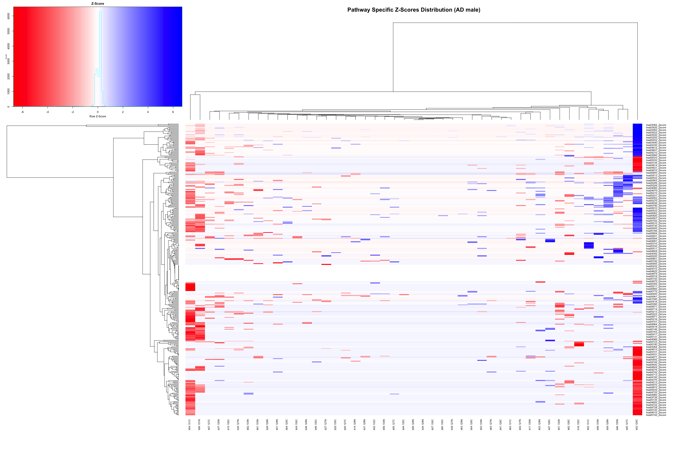
# Convert the data to numeric type (if it's not already)
heatmap_data_AD_male <- as.matrix(heatmap_data_AD_male)

# Define the color palette
color_palette <- colorRampPalette(c("red", "white", "blue"))(100)

# Generate the heatmap
out_heatmap_AD_male <- heatmap.2(
  heatmap_data_AD_male,              # Data matrix
  Rowv = TRUE,                 # Row dendrogram
  Colv = TRUE,                 # Column dendrogram
  col = color_palette,         # Color palette
  scale = "row",              # No scaling
  trace = "none",              # Turn off trace lines
  margins = c(10, 10),         # Set margins for labels
  key = TRUE,                  # Include color key
  key.title = "Z-Score",       # Key title
  keysize = 1.5,               # Size of the key
  cexRow = 0.8,                # Size of row labels
  cexCol = 0.8,                # Size of column labels
  dendrogram = "both",         # Show both row and column dendrograms
  main = "Pathway Specific Z-Scores Distribution (AD male)"  # Main title
)
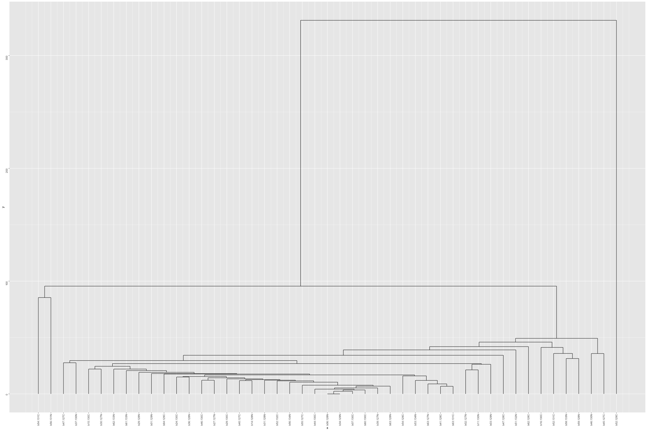
# Plot the dendogram
ggdendrogram(out_heatmap_AD_male$colDendrogram, theme_dendro = FALSE)
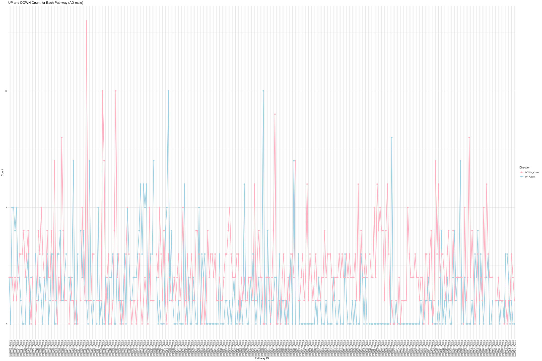
# Convert data from wide to long format
long_sig_pathway_AD_male <- gather(sig_pathway_AD_male, key = "Direction", value = "Count", UP_Count, DOWN_Count)

# Create the line plot
ggplot(long_sig_pathway_AD_male, aes(x = Pathway_ID, y = Count, color = Direction, group = Direction)) +
  geom_line(size = 1) +    # Add lines between points
  geom_point(size = 2) +   # Add points at each Pathway_ID
  theme_minimal() +
  labs(title = "UP and DOWN Count for Each Pathway (AD male)", x = "Pathway ID", y = "Count") +
  theme(axis.text.x = element_text(angle = 90, hjust = 1, size = 8)) +  # Rotate x-axis labels if needed
  scale_color_manual(values = c("UP_Count" = "lightblue", "DOWN_Count" = "pink"))  # Customize colors
## Warning: Removed 16 rows containing missing values or values outside the scale range
## (`geom_point()`).
############################################################################################################################################################################
############################################################################################################################################################################

## AsymAD_female

# Merge both the data frame by Pathway_ID
merged_data_female_AsymAD <- merge(zscored_threshold_female, final_results_AsymAD_female_t, by = "Pathway_ID")

# Initialize an empty data frame to store results
sig_pathway_AsymAD_female <- data.frame(Pathway_ID = merged_data_female_AsymAD$Pathway_ID)

# Iterate over each column in B (excluding the Pathway_ID)
#for (col_name in colnames(final_results_AsymAD_female_t)[-1]) {

  # Apply the conditions and store the result in a new column in Output
  #sig_pathway_AsymAD_female[[col_name]] <- ifelse(merged_data_female_AsymAD[[col_name]] < merged_data_female_AsymAD$lower_1st_percentile,
                               #"DOWN",
                               #ifelse(merged_data_female_AsymAD[[col_name]] > merged_data_female_AsymAD$upper_99th_percentile,
                                      #"UP",
                                      #"0"))
#}

# Add a column to count the number of "UP" occurrences in each row
#sig_pathway_AsymAD_female$UP_Count <- rowSums(sig_pathway_AsymAD_female == "UP")

# Add a column to count the number of "DOWN" occurrences in each row
#sig_pathway_AsymAD_female$DOWN_Count <- rowSums(sig_pathway_AsymAD_female == "DOWN")


# Iterate over each column in final_results_AsymAD_female_t (excluding the Pathway_ID)
for (col_name in colnames(final_results_AsymAD_female_t)[-1]) {

  # Apply the conditions and store the actual value or 0 in a new column in sig_pathway_AsymAD_female
  sig_pathway_AsymAD_female[[col_name]] <- ifelse(
    merged_data_female_AsymAD[[col_name]] < merged_data_female_AsymAD$lower_1st_percentile,
    merged_data_female_AsymAD[[col_name]],  # Retrieve the value if it's less than the lower 1st percentile
    ifelse(
      merged_data_female_AsymAD[[col_name]] > merged_data_female_AsymAD$upper_99th_percentile,
      merged_data_female_AsymAD[[col_name]],  # Retrieve the value if it's greater than the upper 99th percentile
      0  # Otherwise, set to 0
    )
  )
}

# Select only numeric columns (assuming all columns except Pathway_ID are numeric)
numeric_columns <- sig_pathway_AsymAD_female[, sapply(sig_pathway_AsymAD_female, is.numeric)]

# Calculate UP_count (count of positive values) for each row
sig_pathway_AsymAD_female$UP_Count <- rowSums(numeric_columns > 0)

# Calculate DOWN_count (count of negative values) for each row
sig_pathway_AsymAD_female$DOWN_Count <- rowSums(numeric_columns < 0)

# Write the output to a .txt file
write.table(sig_pathway_AsymAD_female, "sig_pathway_AsymAD_female.txt", sep = "\t", quote = FALSE, row.names = FALSE)

# Print the table using DT
datatable(sig_pathway_AsymAD_female, options = list(pageLength = 5, autoWidth = TRUE))

###################################################################################################################################################
# Plot the data

# Remove the UP_Count and DOWN_Count columns
heatmap_data_AsymAD_female <- sig_pathway_AsymAD_female[, !(colnames(sig_pathway_AsymAD_female) %in% c("UP_Count", "DOWN_Count"))]

# Set the row names to Pathway_ID and remove the Pathway_ID column
row.names(heatmap_data_AsymAD_female) <- sig_pathway_AsymAD_female$Pathway_ID
heatmap_data_AsymAD_female$Pathway_ID <- NULL

# Check and handle NA/NaN/Inf values
heatmap_data_AsymAD_female[is.na(heatmap_data_AsymAD_female)] <- 0  # Replace NA values with 0
heatmap_data_AsymAD_female[is.infinite(heatmap_data_AsymAD_female)] <- 0  # Replace Inf/-Inf values with 0
## Error in is.infinite(heatmap_data_AsymAD_female): default method not implemented for type 'list'
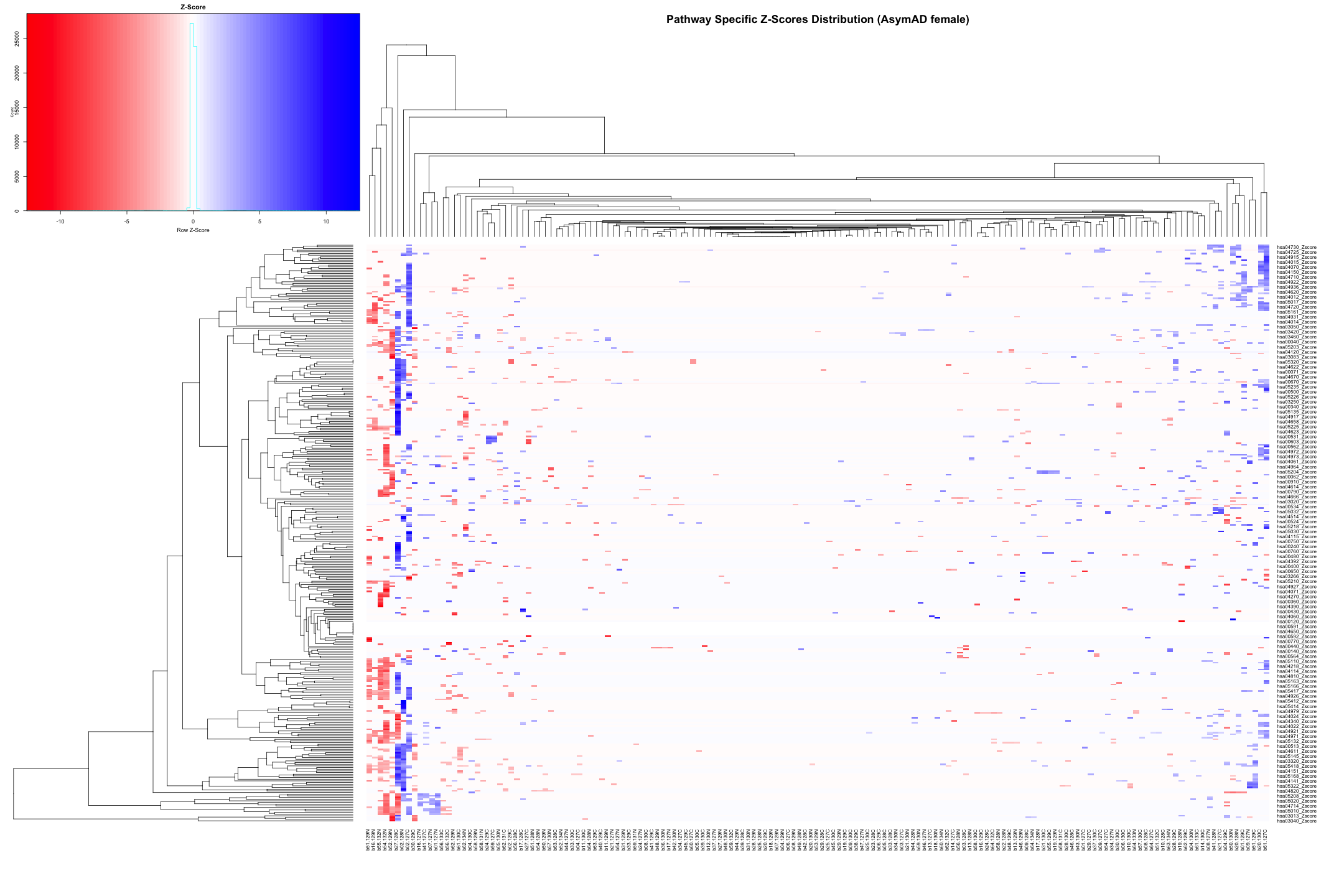
# Convert the data to numeric type (if it's not already)
heatmap_data_AsymAD_female <- as.matrix(heatmap_data_AsymAD_female)

# Define the color palette
color_palette <- colorRampPalette(c("red", "white", "blue"))(100)

# Generate the heatmap
out_heatmap_AsymAD_female <- heatmap.2(
  heatmap_data_AsymAD_female,              # Data matrix
  Rowv = TRUE,                 # Row dendrogram
  Colv = TRUE,                 # Column dendrogram
  col = color_palette,         # Color palette
  scale = "row",              # No scaling
  trace = "none",              # Turn off trace lines
  margins = c(10, 10),         # Set margins for labels
  key = TRUE,                  # Include color key
  key.title = "Z-Score",       # Key title
  keysize = 1.5,               # Size of the key
  cexRow = 0.8,                # Size of row labels
  cexCol = 0.8,                # Size of column labels
  dendrogram = "both",         # Show both row and column dendrograms
  main = "Pathway Specific Z-Scores Distribution (AsymAD female)"  # Main title
)
# Plot the dendogram
ggdendrogram(out_heatmap_AsymAD_female$colDendrogram, theme_dendro = TRUE)
# Convert data from wide to long format
long_sig_pathway_AsymAD_female <- gather(sig_pathway_AsymAD_female, key = "Direction", value = "Count", UP_Count, DOWN_Count)

# Create the bar plot
ggplot(long_sig_pathway_AsymAD_female, aes(x = Pathway_ID, y = Count, color = Direction, group = Direction)) +
  geom_line(size = 1) +    # Add lines between points
  geom_point(size = 2) +   # Add points at each Pathway_ID
  theme_minimal() +
  labs(title = "UP and DOWN Count for Each Pathway (AsymAD female)", x = "Pathway ID", y = "Count") +
  theme(axis.text.x = element_text(angle = 90, hjust = 1, size = 8)) +  # Rotate x-axis labels if needed
  scale_color_manual(values = c("UP_Count" = "lightblue", "DOWN_Count" = "pink"))  # Customize colors
## Warning: Removed 16 rows containing missing values or values outside the scale range
## (`geom_point()`).
############################################################################################################################################################################
############################################################################################################################################################################
## AsymAD_male

# Merge both the data frame by Pathway_ID
merged_data_male_AsymAD <- merge(zscored_threshold_male, final_results_AsymAD_male_t, by = "Pathway_ID")

# Initialize an empty data frame to store results
sig_pathway_AsymAD_male <- data.frame(Pathway_ID = merged_data_male_AsymAD$Pathway_ID)


# Iterate over each column in final_results_AsymAD_female_t (excluding the Pathway_ID)
for (col_name in colnames(final_results_AsymAD_male_t)[-1]) {

  # Apply the conditions and store the actual value or 0 in a new column in sig_pathway_AsymAD_male
  sig_pathway_AsymAD_male[[col_name]] <- ifelse(
    merged_data_male_AsymAD[[col_name]] < merged_data_male_AsymAD$lower_1st_percentile,
    merged_data_male_AsymAD[[col_name]],  # Retrieve the value if it's less than the lower 1st percentile
    ifelse(
      merged_data_male_AsymAD[[col_name]] > merged_data_male_AsymAD$upper_99th_percentile,
      merged_data_male_AsymAD[[col_name]],  # Retrieve the value if it's greater than the upper 99th percentile
      0  # Otherwise, set to 0
    )
  )
}

# Select only numeric columns (assuming all columns except Pathway_ID are numeric)
numeric_columns <- sig_pathway_AsymAD_male[, sapply(sig_pathway_AsymAD_male, is.numeric)]

# Calculate UP_count (count of positive values) for each row
sig_pathway_AsymAD_male$UP_Count <- rowSums(numeric_columns > 0)

# Calculate DOWN_count (count of negative values) for each row
sig_pathway_AsymAD_male$DOWN_Count <- rowSums(numeric_columns < 0)

# Write the output to a .txt file
write.table(sig_pathway_AsymAD_male, "sig_pathway_AsymAD_male.txt", sep = "\t", quote = FALSE, row.names = FALSE)

# Print the table using DT
datatable(sig_pathway_AsymAD_male, options = list(pageLength = 5, autoWidth = TRUE))
###################################################################################################################################################
# Plot the data

# Remove the UP_Count and DOWN_Count columns
heatmap_data_AsymAD_male <- sig_pathway_AsymAD_male[, !(colnames(sig_pathway_AsymAD_male) %in% c("UP_Count", "DOWN_Count"))]

# Set the row names to Pathway_ID and remove the Pathway_ID column
row.names(heatmap_data_AsymAD_male) <- sig_pathway_AsymAD_male$Pathway_ID
heatmap_data_AsymAD_male$Pathway_ID <- NULL

# Check and handle NA/NaN/Inf values
heatmap_data_AsymAD_male[is.na(heatmap_data_AsymAD_male)] <- 0  # Replace NA values with 0
heatmap_data_AsymAD_male[is.infinite(heatmap_data_AsymAD_male)] <- 0  # Replace Inf/-Inf values with 0
## Error in is.infinite(heatmap_data_AsymAD_male): default method not implemented for type 'list'
# Convert the data to numeric type (if it's not already)
heatmap_data_AsymAD_male <- as.matrix(heatmap_data_AsymAD_male)

# Define the color palette
color_palette <- colorRampPalette(c("red", "white", "blue"))(100)

# Generate the heatmap
out_heatmap_AsymAD_male <- heatmap.2(
  heatmap_data_AsymAD_male,              # Data matrix
  Rowv = TRUE,                 # Row dendrogram
  Colv = TRUE,                 # Column dendrogram
  col = color_palette,         # Color palette
  scale = "row",              # No scaling
  trace = "none",              # Turn off trace lines
  margins = c(10, 10),         # Set margins for labels
  key = TRUE,                  # Include color key
  key.title = "Z-Score",       # Key title
  keysize = 1.5,               # Size of the key
  cexRow = 0.8,                # Size of row labels
  cexCol = 0.8,                # Size of column labels
  dendrogram = "both",         # Show both row and column dendrograms
  main = "Pathway Specific Z-Scores Distribution (AsymAD male)"  # Main title
)
# Plot the dendogram
ggdendrogram(out_heatmap_AsymAD_male$colDendrogram, theme_dendro = FALSE)
# Convert data from wide to long format
long_sig_pathway_AsymAD_male <- gather(sig_pathway_AsymAD_male, key = "Direction", value = "Count", UP_Count, DOWN_Count)

# Create the line plot
ggplot(long_sig_pathway_AsymAD_male, aes(x = Pathway_ID, y = Count, color = Direction, group = Direction)) +
  geom_line(size = 1) +    # AsymADd lines between points
  geom_point(size = 2) +   # Add points at each Pathway_ID
  theme_minimal() +
  labs(title = "UP and DOWN Count for Each Pathway (AsymAD male)", x = "Pathway ID", y = "Count") +
  theme(axis.text.x = element_text(angle = 90, hjust = 1, size = 8)) +  # Rotate x-axis labels if needed
  scale_color_manual(values = c("UP_Count" = "lightblue", "DOWN_Count" = "pink"))  # Customize colors
## Warning: Removed 14 rows containing missing values or values outside the scale range
## (`geom_point()`).
############################################################################################################################################################################
############################################################################################################################################################################

## CT_female

# Merge both data frames by Pathway_ID
merged_data_female_CT <- merge(zscored_threshold_female, final_results_CT_female_t, by = "Pathway_ID", all.x = TRUE)

# Initialize an empty data frame to store results
sig_pathway_CT_female <- data.frame(Pathway_ID = merged_data_female_CT$Pathway_ID)

# Iterate over each column in final_results_CT_female_t (excluding the Pathway_ID)
for (col_name in colnames(final_results_CT_female_t)[-1]) {

  # Apply the conditions and store the actual value or 0 in a new column in sig_pathway_CT_female
  sig_pathway_CT_female[[col_name]] <- ifelse(
    merged_data_female_CT[[col_name]] < merged_data_female_CT$lower_1st_percentile,
    merged_data_female_CT[[col_name]],  # Retrieve the value if it's less than the lower 1st percentile
    ifelse(
      merged_data_female_CT[[col_name]] > merged_data_female_CT$upper_99th_percentile,
      merged_data_female_CT[[col_name]],  # Retrieve the value if it's greater than the upper 99th percentile
      0  # Otherwise, set to 0
    )
  )
}

# Select only numeric columns (assuming all columns except Pathway_ID are numeric)
numeric_columns <- sig_pathway_CT_female[, sapply(sig_pathway_CT_female, is.numeric)]

# Calculate UP_count (count of positive values) for each row
sig_pathway_CT_female$UP_Count <- rowSums(numeric_columns > 0)

# Calculate DOWN_count (count of negative values) for each row
sig_pathway_CT_female$DOWN_Count <- rowSums(numeric_columns < 0)

# Write the output to a .txt file
write.table(sig_pathway_CT_female, "sig_pathway_CT_female.txt", sep = "\t", quote = FALSE, row.names = FALSE)

# Print the table using DT
datatable(sig_pathway_CT_female, options = list(pageLength = 5, autoWidth = TRUE))
###################################################################################################################################################
# Plot the data

# Remove the UP_Count and DOWN_Count columns
heatmap_data_CT_female <- sig_pathway_CT_female[, !(colnames(sig_pathway_CT_female) %in% c("UP_Count", "DOWN_Count"))]

# Set the row names to Pathway_ID and remove the Pathway_ID column
row.names(heatmap_data_CT_female) <- sig_pathway_CT_female$Pathway_ID
heatmap_data_CT_female$Pathway_ID <- NULL

# Check and handle NA/NaN/Inf values
heatmap_data_CT_female[is.na(heatmap_data_CT_female)] <- 0  # Replace NA values with 0
heatmap_data_CT_female[is.infinite(heatmap_data_CT_female)] <- 0  # Replace Inf/-Inf values with 0
## Error in is.infinite(heatmap_data_CT_female): default method not implemented for type 'list'
# Convert the data to numeric type (if it's not already)
heatmap_data_CT_female <- as.matrix(heatmap_data_CT_female)

# Define the color palette
color_palette <- colorRampPalette(c("red", "white", "blue"))(100)

# Generate the heatmap
heatmap.2(
  heatmap_data_CT_female,              # Data matrix
  Rowv = TRUE,                 # Row dendrogram
  Colv = TRUE,                 # Column dendrogram
  col = color_palette,         # Color palette
  scale = "row",              # No scaling
  trace = "none",              # Turn off trace lines
  margins = c(10, 10),         # Set margins for labels
  key = TRUE,                  # Include color key
  key.title = "Z-Score",       # Key title
  keysize = 1.5,               # Size of the key
  cexRow = 0.8,                # Size of row labels
  cexCol = 0.8,                # Size of column labels
  dendrogram = "both",         # Show both row and column dendrograms
  main = "Pathway Specific Z-Scores Distribution (CT female)"  # Main title
)
# Convert data from wide to long format
long_sig_pathway_CT_female <- gather(sig_pathway_CT_female, key = "Direction", value = "Count", UP_Count, DOWN_Count)

# Create the bar plot
ggplot(long_sig_pathway_CT_female, aes(x = Pathway_ID, y = Count, fill = Direction)) +
  geom_bar(stat = "identity", position = "dodge") +
  theme_minimal() +
  labs(title = "UP and DOWN Count for Each Pathway (CT female)", x = "Pathway ID", y = "Count") +
  theme(axis.text.x = element_text(angle = 90, hjust = 1, size = 0.5)) +  # Rotate x-axis labels if needed
  scale_fill_manual(values = c("UP_Count" = "lightblue", "DOWN_Count" = "pink"))  # Customize colors
## Warning: Removed 16 rows containing missing values or values outside the scale range
## (`geom_bar()`).
############################################################################################################################################################################
############################################################################################################################################################################

## CT_male

# Merge both data frames by Pathway_ID
merged_data_male_CT <- merge(zscored_threshold_male, final_results_CT_male_t, by = "Pathway_ID", all.x = TRUE)

# Initialize an empty data frame to store results
sig_pathway_CT_male <- data.frame(Pathway_ID = merged_data_male_CT$Pathway_ID)

# Iterate over each column in final_results_CT_female_t (excluding the Pathway_ID)
for (col_name in colnames(final_results_CT_male_t)[-1]) {

  # Apply the conditions and store the actual value or 0 in a new column in sig_pathway_CT_male
  sig_pathway_CT_male[[col_name]] <- ifelse(
    merged_data_male_CT[[col_name]] < merged_data_male_CT$lower_1st_percentile,
    merged_data_male_CT[[col_name]],  # Retrieve the value if it's less than the lower 1st percentile
    ifelse(
      merged_data_male_CT[[col_name]] > merged_data_male_CT$upper_99th_percentile,
      merged_data_male_CT[[col_name]],  # Retrieve the value if it's greater than the upper 99th percentile
      0  # Otherwise, set to 0
    )
  )
}

# Select only numeric columns (assuming all columns except Pathway_ID are numeric)
numeric_columns <- sig_pathway_CT_male[, sapply(sig_pathway_CT_male, is.numeric)]

# Calculate UP_count (count of positive values) for each row
sig_pathway_CT_male$UP_Count <- rowSums(numeric_columns > 0)

# Calculate DOWN_count (count of negative values) for each row
sig_pathway_CT_male$DOWN_Count <- rowSums(numeric_columns < 0)

# Write the output to a .txt file
write.table(sig_pathway_CT_male, "sig_pathway_CT_male.txt", sep = "\t", quote = FALSE, row.names = FALSE)

# Print the table using DT
datatable(sig_pathway_CT_male, options = list(pageLength = 5, autoWidth = TRUE))
###################################################################################################################################################
# Plot the data

# Remove the UP_Count and DOWN_Count columns
heatmap_data_CT_male <- sig_pathway_CT_male[, !(colnames(sig_pathway_CT_male) %in% c("UP_Count", "DOWN_Count"))]

# Set the row names to Pathway_ID and remove the Pathway_ID column
row.names(heatmap_data_CT_male) <- sig_pathway_CT_male$Pathway_ID
heatmap_data_CT_male$Pathway_ID <- NULL

# Check and handle NA/NaN/Inf values
heatmap_data_CT_male[is.na(heatmap_data_CT_male)] <- 0  # Replace NA values with 0
heatmap_data_CT_male[is.infinite(heatmap_data_CT_male)] <- 0  # Replace Inf/-Inf values with 0
## Error in is.infinite(heatmap_data_CT_male): default method not implemented for type 'list'
# Convert the data to numeric type (if it's not already)
heatmap_data_CT_male <- as.matrix(heatmap_data_CT_male)

# Define the color palette
color_palette <- colorRampPalette(c("red", "white", "blue"))(100)

# Generate the heatmap
heatmap.2(
  heatmap_data_CT_male,              # Data matrix
  Rowv = TRUE,                 # Row dendrogram
  Colv = TRUE,                 # Column dendrogram
  col = color_palette,         # Color palette
  scale = "row",              # No scaling
  trace = "none",              # Turn off trace lines
  margins = c(10, 10),         # Set margins for labels
  key = TRUE,                  # Include color key
  key.title = "Z-Score",       # Key title
  keysize = 1.5,               # Size of the key
  cexRow = 0.8,                # Size of row labels
  cexCol = 0.8,                # Size of column labels
  dendrogram = "both",         # Show both row and column dendrograms
  main = "Pathway Specific Z-Scores Distribution (CT male)"  # Main title
)
# Convert data from wide to long format
long_sig_pathway_CT_male <- gather(sig_pathway_CT_male, key = "Direction", value = "Count", UP_Count, DOWN_Count)

# Create the bar plot
ggplot(long_sig_pathway_CT_male, aes(x = Pathway_ID, y = Count, fill = Direction)) +
  geom_bar(stat = "identity", position = "dodge") +
  theme_minimal() +
  labs(title = "UP and DOWN Count for Each Pathway (CT male)", x = "Pathway ID", y = "Count") +
  theme(axis.text.x = element_text(angle = 90, hjust = 1, size = 0.5)) +  # Rotate x-axis labels if needed
  scale_fill_manual(values = c("UP_Count" = "lightblue", "DOWN_Count" = "pink"))  # Customize colors
## Warning: Removed 14 rows containing missing values or values outside the scale range
## (`geom_bar()`).
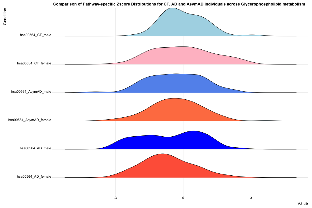
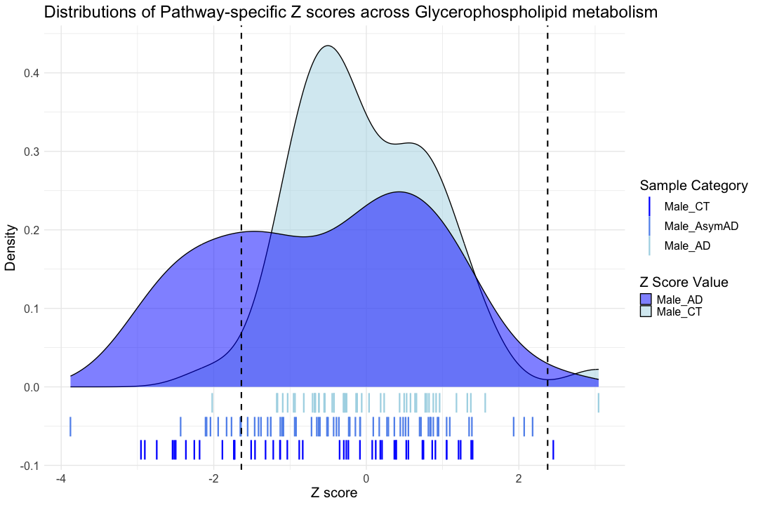
Compare Pathway-specific Zscore Distributions for CT and AD Individuals across Glycerophospholipid metabolism :
library(ggplot2)
library(ggridges)
library(reshape2)
library(ggbreak)
# Select pathway-specific (eg: hsa00564) Zscore from all four groups

# Find the maximum length of the vectors
max_length <- max(
  length(final_results_AD_female$hsa00564_Zscore),
  length(final_results_AD_male$hsa00564_Zscore),
  length(final_results_AsymAD_female$hsa00564_Zscore),
  length(final_results_AsymAD_male$hsa00564_Zscore),
  length(final_results_CT_female$hsa00564_Zscore),
  length(final_results_CT_male$hsa00564_Zscore)
)

# Function to pad a vector with NA values
pad_vector <- function(vec, length_out) {
  c(vec, rep(NA, length_out - length(vec)))
}

# Pad each vector to the maximum length
hsa00564_AD_female_padded <- pad_vector(final_results_AD_female$hsa00564_Zscore, max_length)
hsa00564_AD_male_padded <- pad_vector(final_results_AD_male$hsa00564_Zscore, max_length)
hsa00564_AsymAD_female_padded <- pad_vector(final_results_AsymAD_female$hsa00564_Zscore, max_length)
hsa00564_AsymAD_male_padded <- pad_vector(final_results_AsymAD_male$hsa00564_Zscore, max_length)
hsa00564_CT_female_padded <- pad_vector(final_results_CT_female$hsa00564_Zscore, max_length)
hsa00564_CT_male_padded <- pad_vector(final_results_CT_male$hsa00564_Zscore, max_length)

# Combine into a single data frame
hsa00564_Zscore_summary <- data.frame(
  hsa00564_AD_female = hsa00564_AD_female_padded,
  hsa00564_AD_male = hsa00564_AD_male_padded,
  hsa00564_AsymAD_female = hsa00564_AsymAD_female_padded,
  hsa00564_AsymAD_male = hsa00564_AsymAD_male_padded,
  hsa00564_CT_female = hsa00564_CT_female_padded,
  hsa00564_CT_male = hsa00564_CT_male_padded
)

# View the combined data frame
#head(hsa00564_Zscore_summary)

# Print the table using DT
datatable(hsa00564_Zscore_summary, options = list(pageLength = 5, autoWidth = TRUE))
#write.table(hsa00564_Zscore_summary, "/Users/poddea/Desktop/hsa00564_Zscore_summary.txt", sep = "\t", quote = FALSE, row.names = FALSE)

# Transform the data to long format
hsa00564_Zscore_summary_long <- melt(hsa00564_Zscore_summary, variable.name = "Condition", value.name = "Value")
# Remove NA values (if any)
hsa00564_Zscore_summary_long <- hsa00564_Zscore_summary_long[complete.cases(hsa00564_Zscore_summary_long), ]

# Create the Ridgeline Plot:
ggplot(hsa00564_Zscore_summary_long, aes(x = Value, y = Condition, fill = Condition)) +
  geom_density_ridges(scale = 1) +
  theme_ridges() +
  theme(legend.position = "none") +
  labs(title = "Comparison of Pathway-specific Zscore Distributions for CT, AD and AsymAD Individuals across Glycerophospholipid metabolism ", x = "Value", y = "Condition") +
  scale_fill_manual(values = c("tomato", "blue", "coral", "cornflowerblue", "pink", "lightblue"))
##############################################################################################################################################################

# Filter the data for Female_CT and Female_AD
data_filtered_AD_mf <- subset(hsa00564_Zscore_summary_long, Condition %in% c("hsa00564_AD_female", "hsa00564_AD_male"))

data_filtered_CTAD_m <- subset(hsa00564_Zscore_summary_long, Condition %in% c("hsa00564_CT_male", "hsa00564_AD_male"))

data_filtered_CTAD_f <- subset(hsa00564_Zscore_summary_long, Condition %in% c("hsa00564_CT_female", "hsa00564_AD_female"))

# Create the overlapping density plot
ggplot(data_filtered_AD_mf, aes(x = Value, fill = Condition)) +
  geom_density(alpha = 0.5) +  # Set transparency for overlapping densities
  theme_minimal() +
  labs(title = "Density Plot for AD_male and AD_female across Glycerophospholipid metabolism   pathway",
       x = "Z score",
       y = "Density") +
  scale_fill_manual(values = c("hsa00564_AD_female" = "red", "hsa00564_AD_male" = "blue")) +
  theme_minimal(base_size = 14) +
  theme(
    text = element_text(size = 20),
    legend.position = "right"
  )
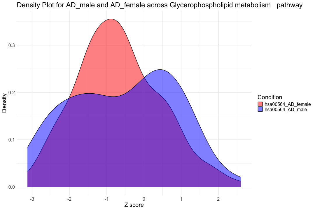
result_AD_mf <- wilcox.test(hsa00564_Zscore_summary$hsa00564_AD_male, hsa00564_Zscore_summary$hsa00564_AD_female, paired = TRUE, na.rm = TRUE)

print(result_AD_mf)
##
## 	Wilcoxon signed rank exact test
##
## data:  hsa00564_Zscore_summary$hsa00564_AD_male and hsa00564_Zscore_summary$hsa00564_AD_female
## V = 669, p-value = 0.2715
## alternative hypothesis: true location shift is not equal to 0
ggplot(data_filtered_CTAD_m, aes(x = Value, fill = Condition)) +
  geom_density(alpha = 0.5) +  # Set transparency for overlapping densities
  theme_minimal() +
  labs(title = "Density Plot for CT_male and AD_male across Glycerophospholipid metabolism   pathway",
       x = "Z score",
       y = "Density") +
  scale_fill_manual(values = c("hsa00564_CT_male" = "lightblue", "hsa00564_AD_male" = "blue")) +
  theme(legend.title = element_blank())
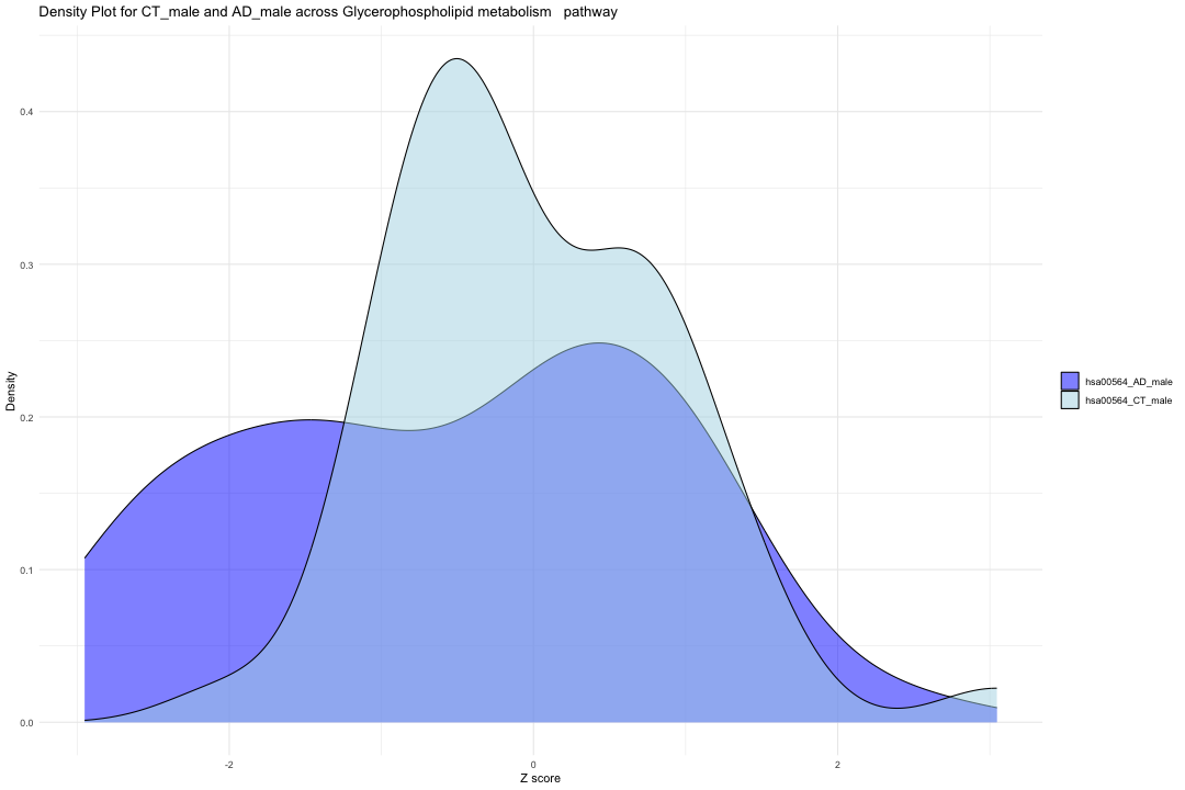
result_CTAD_m <- wilcox.test(hsa00564_Zscore_summary$hsa00564_CT_male, hsa00564_Zscore_summary$hsa00564_AD_male, paired = TRUE, na.rm = TRUE)

print(result_CTAD_m)
##
## 	Wilcoxon signed rank exact test
##
## data:  hsa00564_Zscore_summary$hsa00564_CT_male and hsa00564_Zscore_summary$hsa00564_AD_male
## V = 757, p-value = 0.01727
## alternative hypothesis: true location shift is not equal to 0
ggplot(data_filtered_CTAD_f, aes(x = Value, fill = Condition)) +
  geom_density(alpha = 0.5) +  # Set transparency for overlapping densities
  theme_minimal() +
  labs(title = "Density Plot for CT_female and AD_female across Glycerophospholipid metabolism ",
       x = "Z score",
       y = "Density") +
  scale_fill_manual(values = c("hsa00564_CT_female" = "pink", "hsa00564_AD_female" = "red")) +
  theme(legend.title = element_blank())
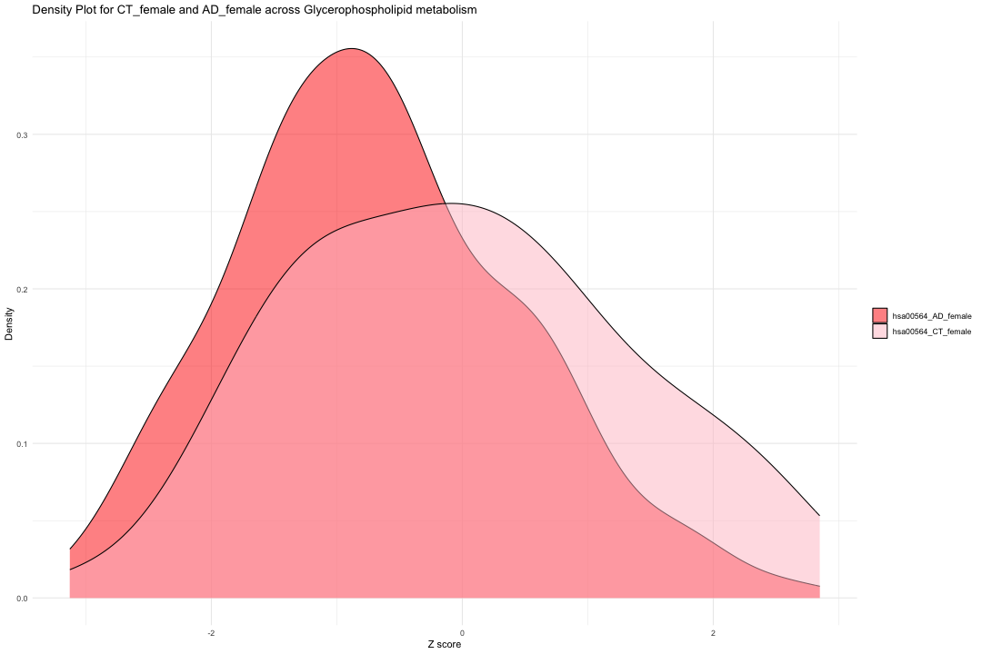
result_CTAD_f <- wilcox.test(hsa00564_Zscore_summary$hsa00564_CT_female, hsa00564_Zscore_summary$hsa00564_AD_female, paired = TRUE, na.rm = TRUE)

print(result_CTAD_f)
##
## 	Wilcoxon signed rank test with continuity correction
##
## data:  hsa00564_Zscore_summary$hsa00564_CT_female and hsa00564_Zscore_summary$hsa00564_AD_female
## V = 1631, p-value = 0.005182
## alternative hypothesis: true location shift is not equal to 0
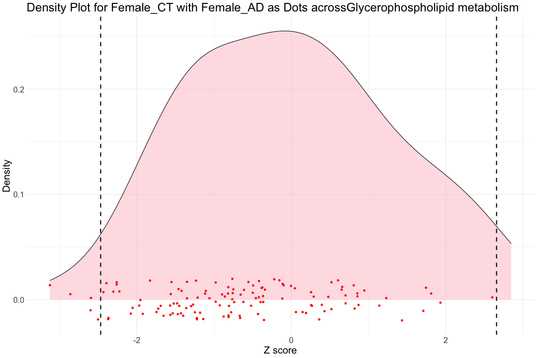
########################################################################################################################################################################

# Calculate the 1st and 99th percentiles of pathway-specific Z scores for the hsa00564 pathway within the Control individuals
hsa00564_CT_female_1st <- quantile(hsa00564_Zscore_summary$hsa00564_CT_female, 0.01, na.rm = TRUE)
hsa00564_CT_female_99th <- quantile(hsa00564_Zscore_summary$hsa00564_CT_female, 0.99, na.rm = TRUE)

hsa00564_CT_male_1st <- quantile(hsa00564_Zscore_summary$hsa00564_CT_male, 0.01, na.rm = TRUE)
hsa00564_CT_male_99th <- quantile(hsa00564_Zscore_summary$hsa00564_CT_male, 0.99, na.rm = TRUE)


ggplot(hsa00564_Zscore_summary, aes(x = hsa00564_CT_female)) +
  geom_density(fill = "pink", alpha = 0.5) +  # Density plot for Female_CT
  geom_point(aes(x = hsa00564_AD_female, y = 0), position = position_jitter(height = 0.02), color = "red") +  # Dots for Female_AD
  labs(title = "Density Plot for Female_CT with Female_AD as Dots acrossGlycerophospholipid metabolism ",
       x = "Z score",
       y = "Density") +
  theme_minimal() +
  geom_vline(xintercept = hsa00564_CT_female_1st, color = "black", linetype = "dashed", size = 1) +
  geom_vline(xintercept = hsa00564_CT_female_99th, color = "black", linetype = "dashed", size = 1) +
  theme(text = element_text(size=20))
## Warning: Removed 91 rows containing non-finite outside the scale range
## (`stat_density()`).
## Warning: Removed 32 rows containing missing values or values outside the scale range
## (`geom_point()`).
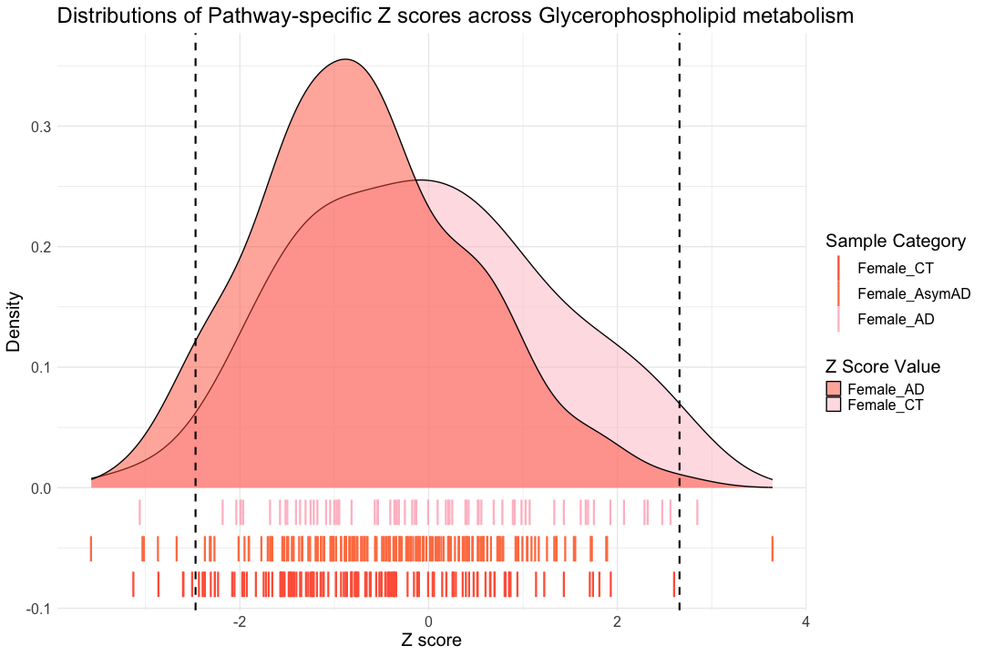
###############################################################################################################################

ggplot() +
  # Density plot for Female_CT
  geom_density(
    data = hsa00564_Zscore_summary,
    aes(x = hsa00564_CT_female, fill = "Female_CT"),
    alpha = 0.5
  ) +
  # Density plot for Female_AD
  geom_density(
    data = hsa00564_Zscore_summary,
    aes(x = hsa00564_AD_female, fill = "Female_AD"),
    alpha = 0.5
  ) +
  # Mimic rug plot for Female_CT
  geom_point(
    data = hsa00564_Zscore_summary,
    aes(x = hsa00564_CT_female, y = -0.02, color = "Female_CT"),
    size = 10, shape = "|"
  ) +
  # Mimic rug plot for Female_AsymAD
  geom_point(
    data = hsa00564_Zscore_summary,
    aes(x = hsa00564_AsymAD_female, y = -0.05, color = "Female_AsymAD"),
    size = 10, shape = "|"
  ) +
    # Mimic rug plot for Female_AD
  geom_point(
    data = hsa00564_Zscore_summary,
    aes(x = hsa00564_AD_female, y = -0.08, color = "Female_AD"),
    size = 10, shape = "|"
  ) +
  # Labels and themes
  labs(
    title = "Distributions of Pathway-specific Z scores across Glycerophospholipid metabolism ",
    x = "Z score",
    y = "Density",
    fill = "Z Score Value",
    color = "Sample Category"
  ) +
  theme_minimal(base_size = 14) +
  theme(
    text = element_text(size = 20),
    legend.position = "right"
  ) +
  # Vertical dashed lines for Female_CT
  geom_vline(xintercept = hsa00564_CT_female_1st, color = "black", linetype = "dashed", size = 1) +
  geom_vline(xintercept = hsa00564_CT_female_99th, color = "black", linetype = "dashed", size = 1) +
  # Manually specify the color scales for the legends
  scale_fill_manual(
    values = c("Female_CT" = "pink", "Female_AD" = "tomato"),
    labels = c("Female_AD", "Female_CT")
  ) +
  scale_color_manual(
    values = c("Female_CT" = "pink","Female_AsymAD" = "coral", "Female_AD" = "tomato"),
    labels = c("Female_CT", "Female_AsymAD", "Female_AD")
  ) #+
## Warning: Removed 91 rows containing non-finite outside the scale range
## (`stat_density()`).
## Warning: Removed 32 rows containing non-finite outside the scale range
## (`stat_density()`).
## Warning: Removed 91 rows containing missing values or values outside the scale range
## (`geom_point()`).
## Warning: Removed 32 rows containing missing values or values outside the scale range
## (`geom_point()`).
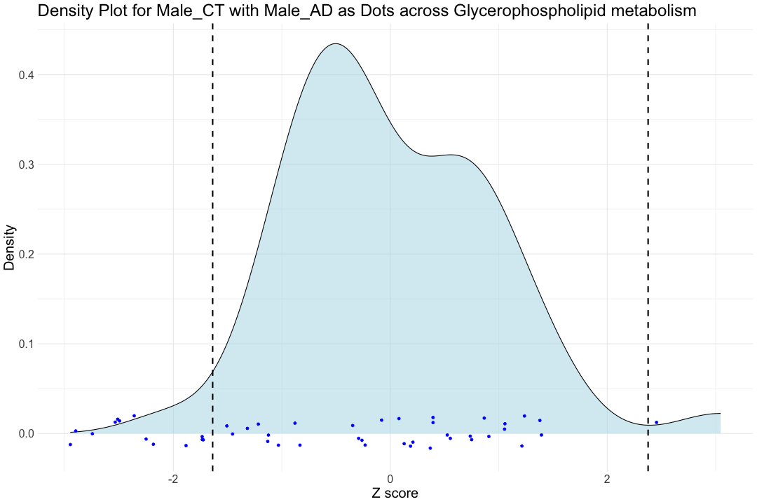
     # Break the X axis manually to make the plot more visible
 #scale_x_break(c(7.5, 17.5), scales = 0.3, ticklabels = c(7.5, 17.5))


###############################################################################################################################

ggplot(hsa00564_Zscore_summary, aes(x = hsa00564_CT_male)) +
  geom_density(fill = "lightblue", alpha = 0.5) +  # Density plot for Female_CT
  geom_point(aes(x = hsa00564_AD_male, y = 0), position = position_jitter(height = 0.02), color = "blue") +  # Dots for Male_AD
  labs(title = "Density Plot for Male_CT with Male_AD as Dots across Glycerophospholipid metabolism ",
       x = "Z score",
       y = "Density") +
  theme_minimal() +
  geom_vline(xintercept = hsa00564_CT_male_1st, color = "black", linetype = "dashed", size = 1) +
  geom_vline(xintercept = hsa00564_CT_male_99th, color = "black", linetype = "dashed", size = 1) +
  theme(text = element_text(size=20))
## Warning: Removed 113 rows containing non-finite outside the scale range
## (`stat_density()`).
## Warning: Removed 112 rows containing missing values or values outside the scale range
## (`geom_point()`).
###############################################################################################################################

ggplot() +
  # Density plot for Male_CT
  geom_density(
    data = hsa00564_Zscore_summary,
    aes(x = hsa00564_CT_male, fill = "Male_CT"),
    alpha = 0.5
  ) +
  # Density plot for Male_AD
  geom_density(
    data = hsa00564_Zscore_summary,
    aes(x = hsa00564_AD_male, fill = "Male_AD"),
    alpha = 0.5
  ) +
  # Mimic rug plot for Male_CT
  geom_point(
    data = hsa00564_Zscore_summary,
    aes(x = hsa00564_CT_male, y = -0.02, color = "Male_CT"),
    size = 10, shape = "|"
  ) +
  # Mimic rug plot for Male_AsymAD
  geom_point(
    data = hsa00564_Zscore_summary,
    aes(x = hsa00564_AsymAD_male, y = -0.05, color = "Male_AsymAD"),
    size = 10, shape = "|"
  ) +
   # Mimic rug plot for Male_AD
  geom_point(
    data = hsa00564_Zscore_summary,
    aes(x = hsa00564_AD_male, y = -0.08, color = "Male_AD"),
    size = 10, shape = "|"
  ) +
  # Labels and themes
  labs(
    title = "Distributions of Pathway-specific Z scores across Glycerophospholipid metabolism ",
    x = "Z score",
    y = "Density",
    fill = "Z Score Value",
    color = "Sample Category"
  ) +
  theme_minimal(base_size = 14) +
  theme(
    text = element_text(size = 20),
    legend.position = "right"
  ) +
  # Vertical dashed lines for Male_CT
  geom_vline(xintercept = hsa00564_CT_male_1st, color = "black", linetype = "dashed", size = 1) +
  geom_vline(xintercept = hsa00564_CT_male_99th, color = "black", linetype = "dashed", size = 1) +
  # Manually specify the color scales for the legends
  scale_fill_manual(
    values = c("Male_CT" = "lightblue", "Male_AD" = "blue"),
    labels = c("Male_AD", "Male_CT")
  ) +
  scale_color_manual(
    values = c("Male_CT" = "lightblue", "Male_AsymAD" = "cornflowerblue",  "Male_AD" = "blue"),
    labels = c("Male_CT", "Male_AsymAD", "Male_AD")
  ) #+
## Warning: Removed 113 rows containing non-finite outside the scale range
## (`stat_density()`).
## Warning: Removed 112 rows containing non-finite outside the scale range
## (`stat_density()`).
## Warning: Removed 113 rows containing missing values or values outside the scale range
## (`geom_point()`).
## Warning: Removed 98 rows containing missing values or values outside the scale range
## (`geom_point()`).
## Warning: Removed 112 rows containing missing values or values outside the scale range
## (`geom_point()`).
   # Break the X axis manually to make the plot more visible
 #scale_x_break(c(10, 20), scales = 0.3, ticklabels = c(10, 20))