Avijit Podder Date: Aug 26, 2024

PHASE 1 and 2 TMT PROTEOMICS MERGED: ROSMAP TMT-proteomics Data (read count file)

library(stringr)
library(dplyr)

## 
## Attaching package: 'dplyr'

## The following objects are masked from 'package:stats':
## 
##     filter, lag

## The following objects are masked from 'package:base':
## 
##     intersect, setdiff, setequal, union

library(ggplot2)

## Warning: package 'ggplot2' was built under R version 4.5.2

library(tidyr)
library(DT)

# Data set: ROSMAP (N=610), Minimally regressed, batch- and set-corrected protein abundance. Batch within set, and inter-set (ROSMAP set1 and set2) correction handled by separate repeats of TAMPOR (proteins kept with <50% missing values within sets); 610 total cases (syn28723003)

protein_data <- read.csv("/Users/poddea/Desktop/ROSMAP_data_100623/TMT_proteomics/Round2/2a.Zero-centered_log2(abundance)-ROSMAP610.R1+R2-2xTAMPORcorrected.csv", sep =",", header = TRUE, stringsAsFactors = FALSE)

dim(protein_data)

## [1] 7814  611

#head(protein_data)

# Split the protein_ID column by "|"
split_protein_data <- str_split_fixed(protein_data$X, "\\|", 2)

# Combine the split data with the original dataframe
protein_data$Protein_name <- split_protein_data[, 1]
protein_data$Uniprot_ID <- split_protein_data[, 2]

# Count the repetitive Protein_name
count_data <- protein_data %>%
  group_by(Protein_name) %>%
  summarise(count = n()) %>%
  filter(count > 1)

# Print the number of repetitive protein_name
cat("Number of repetitive protein_name:", nrow(count_data), "\n")

## Number of repetitive protein_name: 8

# Create a horizontal bar chart
ggplot(count_data, aes(x = reorder(Protein_name, -count), y = count)) +
  geom_bar(stat = "identity", fill = "steelblue") +
  labs(title = "Count of Repetitive protein_names", x = "Protein_name", y = "Count") +
  geom_text(aes(label = count), vjust = -0.5, size = 10) +  # Add text annotations +
  theme_minimal() +
  theme(text = element_text(size=20))

# Find the row (Protein_name) with the highest absolute row sum across all columns for each repetitive Protein_name
protein_data_filtered <- protein_data %>%
  group_by(Protein_name) %>%
  slice(which.max(abs(rowSums(across(starts_with("b"), is.numeric), na.rm = TRUE)))) %>%
  ungroup()

dim(protein_data_filtered)

## [1] 7801  613

#################################################################################################################################################################
## INPUT data File Filtering - Remove proteins without given name (symbol)
## Used "Protein_name as first column in the data file"

# Filter rows where Protein_name is not 0
protein_data_filtered <- protein_data_filtered[protein_data_filtered$Protein_name != "0", ]

# Print the number of IDs with protein_name
cat("Number of IDs with protein_name:", nrow(protein_data_filtered), "\n")

## Number of IDs with protein_name: 7800

# Remove the Uniprot_ID column
protein_data_filtered$Uniprot_ID <- NULL

# Replace the first column with Protein_name
#protein_data_filtered$X <- protein_data_filtered$Protein_name

# Move Protein_name to the first column
protein_data_filtered <- protein_data_filtered[, c("Protein_name", setdiff(names(protein_data_filtered), "Protein_name"))]

# Remove the "X" column
protein_data_filtered$X <- NULL


dim(protein_data_filtered)

## [1] 7800  611

# Print the table using DT
datatable(protein_data_filtered, options = list(pageLength = 5, autoWidth = TRUE))

## Warning in instance$preRenderHook(instance): It seems your data is too big for
## client-side DataTables. You may consider server-side processing:
## https://rstudio.github.io/DT/server.html

PHASE 1 and 2 TMT PROTEOMICS MERGED: ROSMAP TMT-proteomics Metadata (samples description file)

library(stringr)
library(dplyr)
library(ggplot2)
library(tidyr)
library(DT)

# Read the TMT metadata file for ROSMAP individuals
protein_metadata_ROSMAP <- read.csv("/Users/poddea/Desktop/ROSMAP_data_100623/TMT_proteomics/Round2/2c.traits-ROSMAP610.R1+R2-2xTAMPORcorrected.csv", sep =",", header = TRUE, stringsAsFactors = FALSE)

#protein_metadata_ROSMAP <- read.table("/Users/poddea/Desktop/ROSMAP_data_100623/TMT_proteomics/Round2/ROSMAP_Covariates_ages_censored.tsv", sep ="\t", header = TRUE, stringsAsFactors = FALSE)

dim(protein_metadata_ROSMAP)

## [1] 610  41

# Define the catagory (diagnosis) based on the braaksc, CERAD and cogdx
#protein_metadata_ROSMAP$category <- with(protein_metadata_ROSMAP, ifelse(braaksc >= 4 & ceradsc_RADCnonStd <= 2 & cogdx == 4, "AD",
                               #ifelse(braaksc <= 3 & ceradsc_RADCnonStd >= 3 & cogdx == 1, "CT", "OTHER")))


# Define the category based on Braak, CERAD, and MMSE (cognitive status)
protein_metadata_ROSMAP$category <- with(protein_metadata_ROSMAP,
    ifelse((CERAD %in% 0:1 & braaksc %in% 0:2 & cts_mmse30_lv >= 24) |
           (CERAD == 0 & braaksc == 3 & cts_mmse30_lv >= 24), "Control",
    ifelse(CERAD %in% 1:3 & braaksc %in% 3:6 & cts_mmse30_lv >= 24, "AsymAD",
    ifelse(CERAD %in% 2:3 & braaksc %in% 3:6 & cts_mmse30_lv < 24, "AD", "Exclude"))))


# Define the category based on Braak, CERAD, and MMSE (cognitive status)
#protein_metadata_ROSMAP$category <- with(protein_metadata_ROSMAP, 
    #ifelse((CERAD %in% 0:1 & braaksc %in% 0:2 & cts_mmse30_lv >= 24) | 
           #(CERAD == 0 & braaksc == 3 & cts_mmse30_lv >= 24), "Control",
    #ifelse(CERAD %in% 1:3 & braaksc %in% 3:6 & cts_mmse30_lv >= 24, "AsymAD",
    #ifelse(CERAD %in% 2:3 & braaksc %in% 3:6 & cts_mmse30_lv < 24, "AD", "Exclude"))))


# Define the sex_type (sex) based on the msex value
protein_metadata_ROSMAP$sex <- with(protein_metadata_ROSMAP, ifelse(msex == 0, "female",
                                ifelse(msex == 1, "male", "NA")))

write.table(protein_metadata_ROSMAP,"Protein_metadata_ROSMAP_catagory.txt",sep="\t",quote=F)


# Print the table using DT
datatable(protein_metadata_ROSMAP, options = list(pageLength = 5, autoWidth = TRUE))

# Read the outliers file
outliers <- read.table("/Users/poddea/Desktop/ROSMAP_data_100623/TMT_proteomics/Round2/outliers.txt", header = TRUE)

# Extract the IDs to be removed
ids_to_remove <- outliers$Outliers

ids_to_remove

## [1] "b22.130N" "b52.130N" "b56.131C"

# Remove the specified columns from the TMT read count file
protein_data_filtered <- protein_data_filtered[, !colnames(protein_data_filtered) %in% ids_to_remove]

dim(protein_data_filtered)

## [1] 7800  608

# Use the 'subset' function to remove rows with specified IDs (outliers) from the protein_metadata_ROSMAP
protein_metadata_ROSMAP <- subset(protein_metadata_ROSMAP, !(batch.channel %in% ids_to_remove))

dim(protein_metadata_ROSMAP)

## [1] 607  43

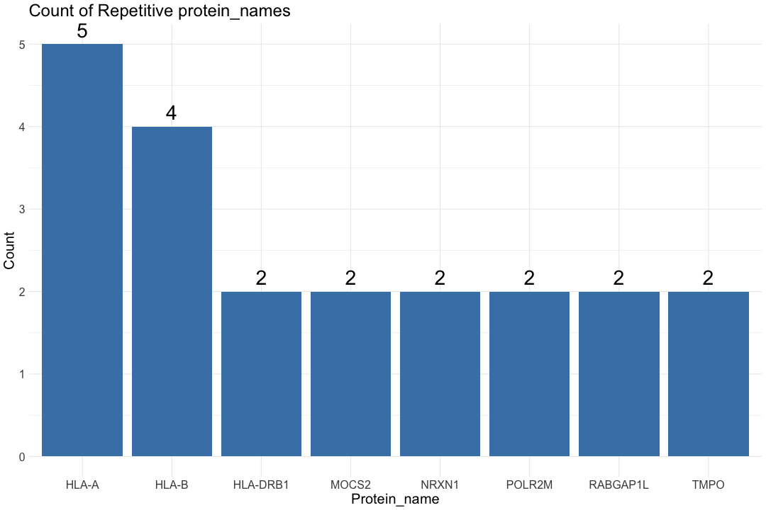
# Get the list of proteins from the protein_data_filtered
Protein_name <- protein_data_filtered$Protein_name

# Get the list of samples from the protein_data_filtered
common_samples <- colnames(protein_data_filtered)

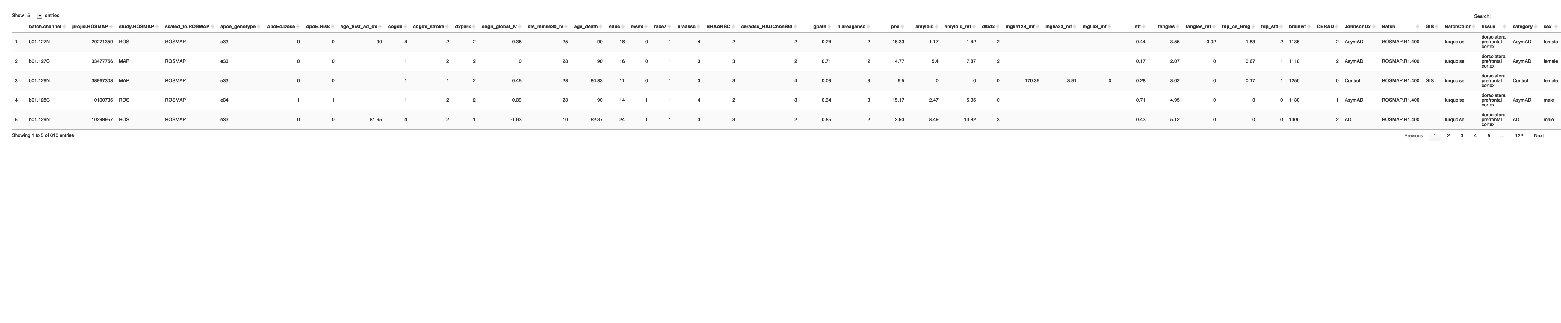
# Select a sub-set of the sample (Tissue: DLPFC) from protein_metadata_ROSMAP file
sample_data_DLPFC <- filter(protein_metadata_ROSMAP, tissue == "dorsolateral prefrontal cortex")

# Create a subset of the DLPFC sample description file with control samples only
sample_data_DLPFC_contorl <- sample_data_DLPFC[grep("Control", sample_data_DLPFC$JohnsonDx), ]

dim(sample_data_DLPFC_contorl)

## [1] 114  43

# Create a subset of the DLPFC sample description file with AD samples only
#sample_data_DLPFC_case <- sample_data_DLPFC[grep("AD", sample_data_DLPFC$JohnsonDx), ]
sample_data_DLPFC_case <- sample_data_DLPFC[sample_data_DLPFC$JohnsonDx == "AD", ]

dim(sample_data_DLPFC_case)

## [1] 174  43

# Create a subset of the DLPFC sample description file with AsymAD samples only
sample_data_DLPFC_AsymAD <- sample_data_DLPFC[grep("AsymAD", sample_data_DLPFC$JohnsonDx), ]

dim(sample_data_DLPFC_AsymAD)

## [1] 220  43

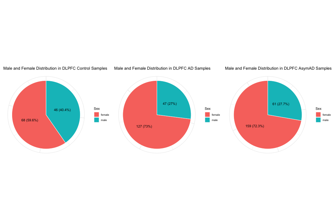
# Calculate the counts and percentages of each sex in control samples
sex_counts_control <- table(sample_data_DLPFC_contorl$sex)
sex_percentages_control <- prop.table(sex_counts_control) * 100

# Create a pie chart to show the distribution of Male and Female ratio within the control samples
pie_data_control <- data.frame(sex = names(sex_counts_control), count = as.numeric(sex_counts_control), percentage = sex_percentages_control)

P1 <- ggplot(pie_data_control, aes(x = "", y = count, fill = sex)) +
  geom_bar(stat = "identity", width = 1, color = "white") +
  coord_polar("y") +
  geom_text(aes(label = paste0(count, " (", round(sex_percentages_control, 1), "%)")), position = position_stack(vjust = 0.5)) +  # Add text labels with percentages
  labs(title = "Male and Female Distribution in DLPFC Control Samples",
       fill = "Sex") +
  theme_minimal() +
  theme(axis.text = element_blank(),
        axis.title = element_blank(),
        legend.position = "right")


# Calculate the counts and percentages of each sex in AD samples
sex_counts_case <- table(sample_data_DLPFC_case$sex)
sex_percentages_case <- prop.table(sex_counts_case) * 100

# Create a pie chart to show the distribution of Male and Female ratio within the AD samples
pie_data_case <- data.frame(sex = names(sex_counts_case), count = as.numeric(sex_counts_case), percentage = sex_percentages_case)

P2 <- ggplot(pie_data_case, aes(x = "", y = count, fill = sex)) +
  geom_bar(stat = "identity", width = 1, color = "white") +
  coord_polar("y") +
  geom_text(aes(label = paste0(count, " (", round(sex_percentages_case, 1), "%)")), position = position_stack(vjust = 0.5)) +  # Add text labels with percentages
  labs(title = "Male and Female Distribution in DLPFC AD Samples",
       fill = "Sex") +
  theme_minimal() +
  theme(axis.text = element_blank(),
        axis.title = element_blank(),
        legend.position = "right")


# Calculate the counts and percentages of each sex in AsymAD samples
sex_counts_AsymAD <- table(sample_data_DLPFC_AsymAD$sex)
sex_percentages_AsymAD <- prop.table(sex_counts_AsymAD) * 100

# Create a pie chart to show the distribution of Male and Female ratio within the AsymAD samples
pie_data_AsymAD <- data.frame(sex = names(sex_counts_AsymAD), count = as.numeric(sex_counts_AsymAD), percentage = sex_percentages_AsymAD)

P3 <- ggplot(pie_data_AsymAD, aes(x = "", y = count, fill = sex)) +
  geom_bar(stat = "identity", width = 1, color = "white") +
  coord_polar("y") +
  geom_text(aes(label = paste0(count, " (", round(sex_percentages_AsymAD, 1), "%)")), position = position_stack(vjust = 0.5)) +  # Add text labels with percentages
  labs(title = "Male and Female Distribution in DLPFC AsymAD Samples",
       fill = "Sex") +
  theme_minimal() +
  theme(axis.text = element_blank(),
        axis.title = element_blank(),
        legend.position = "right")

library(patchwork)

P1 | P2 | P3

Data Missingness calculation (DLPFC Sample Only) - exclude proteins with more than 50% missingness throughout the DLPFC Sample

library(ggplot2)
library(dplyr)
library(ComplexHeatmap)

## Warning: package 'ComplexHeatmap' was built under R version 4.5.1

## Loading required package: grid

## ========================================
## ComplexHeatmap version 2.24.1
## Bioconductor page: http://bioconductor.org/packages/ComplexHeatmap/
## Github page: https://github.com/jokergoo/ComplexHeatmap
## Documentation: http://jokergoo.github.io/ComplexHeatmap-reference
## 
## If you use it in published research, please cite either one:
## - Gu, Z. Complex Heatmap Visualization. iMeta 2022.
## - Gu, Z. Complex heatmaps reveal patterns and correlations in multidimensional 
##     genomic data. Bioinformatics 2016.
## 
## 
## The new InteractiveComplexHeatmap package can directly export static 
## complex heatmaps into an interactive Shiny app with zero effort. Have a try!
## 
## This message can be suppressed by:
##   suppressPackageStartupMessages(library(ComplexHeatmap))
## ========================================

library(circlize)

## ========================================
## circlize version 0.4.16
## CRAN page: https://cran.r-project.org/package=circlize
## Github page: https://github.com/jokergoo/circlize
## Documentation: https://jokergoo.github.io/circlize_book/book/
## 
## If you use it in published research, please cite:
## Gu, Z. circlize implements and enhances circular visualization
##   in R. Bioinformatics 2014.
## 
## This message can be suppressed by:
##   suppressPackageStartupMessages(library(circlize))
## ========================================

library(factoextra)

## Welcome! Want to learn more? See two factoextra-related books at https://goo.gl/ve3WBa

library(grid)

## Filter DLPFC samples from the data

# Select a sub-set of the sample (Tissue: DLPFC) from protein_metadata_ROSMAP file
sample_data_DLPFC <- filter(protein_metadata_ROSMAP, tissue == "dorsolateral prefrontal cortex")

dim(sample_data_DLPFC)

## [1] 607  43

# Create a list of DLPFC samples only
DLPFC_samples <- sample_data_DLPFC$batch.channel

# Create a subset of the protein abundant file with CT samples only
protein_data_DLPFC <- protein_data_filtered[, intersect(common_samples, DLPFC_samples)]

protein_data_DLPFC <- cbind(Protein_name, protein_data_DLPFC)

dim(protein_data_DLPFC)

## [1] 7800  608

# Step 1: Calculate the percentage of missing values (NA) for each row

protein_data_DLPFC <- protein_data_DLPFC %>%
  rowwise() %>%
  mutate(missingness = sum(is.na(c_across(-Protein_name))) / (ncol(.) - 1) * 100)

# Step 2: Filter out rows with more than 50% missingness and store the excluded rows
excluded_protein_count <- protein_data_DLPFC %>%
  filter(missingness > 50)

cat("Total number of Protein_name entries excluded due to more than 50% missing values:", nrow(excluded_protein_count), "\n")

## Total number of Protein_name entries excluded due to more than 50% missing values: 0

# Step 3: Create the filtered dataset with valid rows
protein_data_DLPFC <- protein_data_DLPFC %>%
  filter(missingness <= 50) %>%
  select(-missingness)  #  remove the 'missingness' column from the data

dim(protein_data_DLPFC)

## [1] 7800  608

############################################################################################################################################################
##Calculate the missingness for samples

# Remove the  "Protein_name" column from the file
protein_data_DLPFC_missingness <- protein_data_DLPFC[, -1]

#write.table(protein_data_ROSMAP_new,"/Users/poddea/Desktop/protein_data_ROSMAP_new.txt",sep="\t",quote=T)

# Transpose gene expression data to have samples as rows
protein_data_DLPFC_missingness_missingness_t <- t(protein_data_DLPFC_missingness)

dim(protein_data_DLPFC_missingness_missingness_t)

## [1]  607 7800

# Calculate the number of NA values in each row
na_counts_sample <- apply(protein_data_DLPFC_missingness_missingness_t, 1, function(x) sum(is.na(x)))

# Count the number of rows with at least one NA value
num_samples_with_na <- sum(na_counts_sample > 0)

# Print the total number of rows with at least one NA value
cat("Total number of sample with at least one NA value:", num_samples_with_na, "\n")

## Total number of sample with at least one NA value: 607

# Create a barplot for the NA counts with adjusted margins
barplot(na_counts_sample, main = "Number of missing values (protein abundance) in each individual",
        xlab = "Sample IDs",
        ylab = "Number of missing Proteins",
        col = "blue",
        las = 2,
        cex.names = 0.5)

# Sort the data based on the Y-axis values (na_counts_freq) in descending order
sorted_indices <- order(na_counts_sample, decreasing = TRUE)
na_counts_freq_sorted <- na_counts_sample[sorted_indices]
bar_positions_sorted <- bar_positions[sorted_indices]

## Error: object 'bar_positions' not found

# Create the barplot with the sorted data
barplot(na_counts_freq_sorted,
        main = "Number of missing values (protein abundance) in each individual",
        xlab = "Sample IDs",
        ylab = "Number of missing Proteins",
        col = "blue",
        las = 2,
        cex.names = 0.5)

############################################################################################################################################################

##Calculate the missingness for Protein

# Remove the first row "Protein_name" from the file
protein_data_DLPFC_missingness <- protein_data_DLPFC[-1, ]

# Calculate the number of NA values in each row
na_counts_genes <- apply(protein_data_DLPFC_missingness, 1, function(x) sum(is.na(x)))

# Count the number of rows with at least one NA value
num_genes_with_na <- sum(na_counts_genes > 0)

# Print the total number of rows with at least one NA value
cat("Total number of gene with at least one NA value:", num_genes_with_na, "\n")

## Total number of gene with at least one NA value: 2907

# Count the frequency of each unique NA value
na_counts_freq <- table(na_counts_genes)

#write.table(na_counts_freq,"/Users/poddea/Desktop/na_counts_freq.txt",sep="\t",quote=F)

# Remove the entry for 0 NAs
na_counts_freq <- na_counts_freq[names(na_counts_freq) != "0"]


# Create the barplot and store the bar positions
bar_positions <- barplot(na_counts_freq,
                         main = "Frequency of Individual Counts per Protein",
                         xlab = "Number of missing Protein",
                         ylab = "Frequency of Individual with Missing Protein",
                         col = "blue",
                         las = 2,
                         cex.names = 0.8)

# Sort the data based on the Y-axis values (na_counts_freq) in descending order
sorted_indices <- order(na_counts_freq, decreasing = TRUE)
na_counts_freq_sorted <- na_counts_freq[sorted_indices]
bar_positions_sorted <- bar_positions[sorted_indices]

# Create the barplot with the sorted data
barplot(na_counts_freq_sorted,
        main = "Frequency of Individual Counts per Protein",
        xlab = "Number of missing Protein",
        ylab = "Frequency of Individual with Missing Protein",
        col = "blue",
        las = 2,
        cex.names = 0.8)

############################################################################################################################################################

## Sample-to-Sample distance matrix

protein_data_DLPFC_new <- protein_data_DLPFC[, -1]

# Transpose the protein abundant file to get sample_IDs in the rows
protein_data_DLPFC_t <- t(protein_data_DLPFC_new)

dim(protein_data_DLPFC_t)

## [1]  607 7800

# Compute the Sample-to-Sample Distance Matrix using Euclidean distance
distance_matrix <- dist(protein_data_DLPFC_t)

# Convert the distance matrix to a data frame
distance_df <- as.data.frame(as.matrix(distance_matrix))

write.table(distance_df,"distance_matrix.txt",sep="\t",quote=FALSE, row.names=TRUE)

max(distance_df)

## [1] 76.10121

# Preparing a column annotation file 
col_ha = HeatmapAnnotation(
diagnosis = sample_data_DLPFC$JohnsonDx,
sex = sample_data_DLPFC$sex,
annotation_height = unit(c(12, 12), "cm"),
col = list(
    diagnosis = c("AD" = "purple", "Control" = "lightgreen", "AsymAD" = "royalblue", "Exclude" = "gray47"),
    sex = c("male" = "lightblue", "female" = "lightpink")
  )
)


# Create the heatmap object
ht <- Heatmap(
  as.matrix(distance_matrix),
  name = "Sample-to-Sample Distance Matrix for DLPFC Sample Only",
  top_annotation = col_ha,
  row_names_gp =  gpar(fontsize = 10),  # Top 10 rows larger
  column_names_gp = gpar(fontsize = 5)
  )

## The automatically generated colors map from the 1^st and 99^th of the
## values in the matrix. There are outliers in the matrix whose patterns
## might be hidden by this color mapping. You can manually set the color
## to `col` argument.
## 
## Use `suppressMessages()` to turn off this message.

# Draw the heatmap
draw(ht)

library(gplots)

## 
## Attaching package: 'gplots'

## The following object is masked from 'package:stats':
## 
##     lowess

## Filter CONTROL-FEMALE samples from the data

# Create a list of DLPFC control (female) samples only
DLPFC_CT_samples_female <- sample_data_DLPFC$batch.channel[sample_data_DLPFC$JohnsonDx == "Control" & sample_data_DLPFC$sex == "female"]

# Create a subset of the protein abundant file with CT (female) samples only
protein_data_DLPFC_CT_female <- protein_data_DLPFC[, intersect(common_samples, DLPFC_CT_samples_female)]

protein_data_DLPFC_CT_female <- cbind(Protein_name, protein_data_DLPFC_CT_female)

dim(protein_data_DLPFC_CT_female)

## [1] 7800   69

write.table(protein_data_DLPFC_CT_female,"protein_data_DLPFC_CT_female.txt",sep="\t",quote=FALSE, row.names=FALSE)

datatable(protein_data_DLPFC_CT_female, options = list(pageLength = 5, autoWidth = TRUE))

## Warning in instance$preRenderHook(instance): It seems your data is too big for
## client-side DataTables. You may consider server-side processing:
## https://rstudio.github.io/DT/server.html

# Create a subset of the description file with CT samples only
sample_data_DLPFC_CT <- sample_data_DLPFC[grep("Control", sample_data_DLPFC$JohnsonDx), ]

# Create a subset of the CT sample description file with female samples only
sample_data_DLPFC_CT_female <- sample_data_DLPFC_CT[grep("female", sample_data_DLPFC_CT$sex), ]

dim(sample_data_DLPFC_CT_female)

## [1] 68 43

#########################################################################################################################################

## Filter CONTROL-MALE samples from the data

# Create a list of DLPFC CT (male) samples only
DLPFC_CT_samples_male <- sample_data_DLPFC$batch.channel[sample_data_DLPFC$JohnsonDx == "Control" & sample_data_DLPFC$sex == "male"]

# Create a subset of the protein abundant file with CT (male) samples only
protein_data_DLPFC_CT_male <- protein_data_DLPFC[, intersect(common_samples, DLPFC_CT_samples_male)]

protein_data_DLPFC_CT_male <- cbind(Protein_name, protein_data_DLPFC_CT_male)

dim(protein_data_DLPFC_CT_male)

## [1] 7800   47

write.table(protein_data_DLPFC_CT_male,"protein_data_DLPFC_CT_male.txt",sep="\t",quote=FALSE, row.names=FALSE)

datatable(protein_data_DLPFC_CT_male, options = list(pageLength = 5, autoWidth = TRUE))

## Warning in instance$preRenderHook(instance): It seems your data is too big for
## client-side DataTables. You may consider server-side processing:
## https://rstudio.github.io/DT/server.html

# Create a subset of the description file with CT samples only
sample_data_DLPFC_CT <- sample_data_DLPFC[grep("Control", sample_data_DLPFC$JohnsonDx), ]

# Create a subset of the CT sample description file with male samples only
sample_data_DLPFC_CT_male <- sample_data_DLPFC_CT[sample_data_DLPFC_CT$sex == "male", ]

dim(sample_data_DLPFC_CT_male)

## [1] 46 43

#########################################################################################################################################

## Filter AD-FEMALE samples from the data

# Create a listof DLPFC AD (female) samples only
DLPFC_AD_samples_female <- sample_data_DLPFC$batch.channel[sample_data_DLPFC$JohnsonDx == "AD" & sample_data_DLPFC$sex == "female"]

# Create a subset of the protein abundant file with AD (female) samples only
protein_data_DLPFC_AD_female <- protein_data_DLPFC[, intersect(common_samples, DLPFC_AD_samples_female)]

protein_data_DLPFC_AD_female <- cbind(Protein_name, protein_data_DLPFC_AD_female)

dim(protein_data_DLPFC_AD_female)

## [1] 7800  128

write.table(protein_data_DLPFC_AD_female,"protein_data_DLPFC_AD_female.txt",sep="\t",quote=FALSE, row.names=FALSE)

datatable(protein_data_DLPFC_AD_female, options = list(pageLength = 5, autoWidth = TRUE))

## Warning in instance$preRenderHook(instance): It seems your data is too big for
## client-side DataTables. You may consider server-side processing:
## https://rstudio.github.io/DT/server.html

# Create a subset of the description file with AD samples only
sample_data_DLPFC_AD <- sample_data_DLPFC[sample_data_DLPFC$JohnsonDx == "AD", ]

# Create a subset of the AD sample description file with female samples only
sample_data_DLPFC_AD_female <- sample_data_DLPFC_AD[grep("female", sample_data_DLPFC_AD$sex), ]

dim(sample_data_DLPFC_AD_female)

## [1] 127  43

#########################################################################################################################################

## Filter AD-MALE samples from the data

# Create a listof DLPFC AD (male) samples only
DLPFC_AD_samples_male <- sample_data_DLPFC$batch.channel[sample_data_DLPFC$JohnsonDx == "AD" & sample_data_DLPFC$sex == "male"]

# Create a subset of the protein abundant file with AD (male) samples only
protein_data_DLPFC_AD_male <- protein_data_DLPFC[, intersect(common_samples, DLPFC_AD_samples_male)]

protein_data_DLPFC_AD_male <- cbind(Protein_name, protein_data_DLPFC_AD_male)

dim(protein_data_DLPFC_AD_male)

## [1] 7800   48

write.table(protein_data_DLPFC_AD_male,"protein_data_DLPFC_AD_male.txt",sep="\t",quote=FALSE, row.names=FALSE)

datatable(protein_data_DLPFC_AD_male, options = list(pageLength = 5, autoWidth = TRUE))

## Warning in instance$preRenderHook(instance): It seems your data is too big for
## client-side DataTables. You may consider server-side processing:
## https://rstudio.github.io/DT/server.html

# Create a subset of the description file with AD samples only
sample_data_DLPFC_AD <- sample_data_DLPFC[sample_data_DLPFC$JohnsonDx == "AD", ]

# Create a subset of the AD sample description file with male samples only
sample_data_DLPFC_AD_male <- sample_data_DLPFC_AD[sample_data_DLPFC_AD$sex == "male", ]

dim(sample_data_DLPFC_AD_male)

## [1] 47 43

#########################################################################################################################################

## Filter AsymAD-FEMALE samples from the data

# Create a listof DLPFC AsymAD (female) samples only
DLPFC_AsymAD_samples_female <- sample_data_DLPFC$batch.channel[sample_data_DLPFC$JohnsonDx == "AsymAD" & sample_data_DLPFC$sex == "female"]

# Create a subset of the protein abundant file with AsymAD (female) samples only
protein_data_DLPFC_AsymAD_female <- protein_data_DLPFC[, intersect(common_samples, DLPFC_AsymAD_samples_female)]

protein_data_DLPFC_AsymAD_female <- cbind(Protein_name, protein_data_DLPFC_AsymAD_female)

dim(protein_data_DLPFC_AsymAD_female)

## [1] 7800  160

write.table(protein_data_DLPFC_AsymAD_female,"protein_data_DLPFC_AsymAD_female.txt",sep="\t",quote=FALSE, row.names=FALSE)

datatable(protein_data_DLPFC_AsymAD_female, options = list(pageLength = 5, autoWidth = TRUE))

## Warning in instance$preRenderHook(instance): It seems your data is too big for
## client-side DataTables. You may consider server-side processing:
## https://rstudio.github.io/DT/server.html

# Create a subset of the description file with AsymAD samples only
sample_data_DLPFC_AsymAD <- sample_data_DLPFC[sample_data_DLPFC$JohnsonDx == "AsymAD", ]

# Create a subset of the AsymAD sample description file with female samples only
sample_data_DLPFC_AsymAD_female <- sample_data_DLPFC_AsymAD[grep("female", sample_data_DLPFC_AsymAD$sex), ]

dim(sample_data_DLPFC_AsymAD_female)

## [1] 159  43

#########################################################################################################################################

## Filter AsymAD-MALE samples from the data

# Create a listof DLPFC AsymAD (male) samples only
DLPFC_AsymAD_samples_male <- sample_data_DLPFC$batch.channel[sample_data_DLPFC$JohnsonDx == "AsymAD" & sample_data_DLPFC$sex == "male"]

# Create a subset of the protein abundant file with AsymAD (male) samples only
protein_data_DLPFC_AsymAD_male <- protein_data_DLPFC[, intersect(common_samples, DLPFC_AsymAD_samples_male)]

protein_data_DLPFC_AsymAD_male <- cbind(Protein_name, protein_data_DLPFC_AsymAD_male)

dim(protein_data_DLPFC_AsymAD_male)

## [1] 7800   62

write.table(protein_data_DLPFC_AsymAD_male,"protein_data_DLPFC_AsymAD_male.txt",sep="\t",quote=FALSE, row.names=FALSE)


datatable(protein_data_DLPFC_AsymAD_male, options = list(pageLength = 5, autoWidth = TRUE))

## Warning in instance$preRenderHook(instance): It seems your data is too big for
## client-side DataTables. You may consider server-side processing:
## https://rstudio.github.io/DT/server.html

# Create a subset of the description file with AsymAD samples only
sample_data_DLPFC_AsymAD <- sample_data_DLPFC[sample_data_DLPFC$JohnsonDx == "AsymAD", ]

# Create a subset of the AsymAD sample description file with male samples only
sample_data_DLPFC_AsymAD_male <- sample_data_DLPFC_AsymAD[sample_data_DLPFC_AsymAD$sex == "male", ]

dim(sample_data_DLPFC_AsymAD_male)

## [1] 61 43

Calculating AD and AsymAD Samples Specific Z-score by Averaging the Control Gruop

library(ggplot2)
library(RColorBrewer)
library(scales)
library(gplots)
library(dplyr)
library(tidyr)

## Function to calculate MEAN and SD for each gene within the Control Female samples

# Calculation of MEAN for each row
protein_data_DLPFC_CT_female$MEAN <- rowMeans(protein_data_DLPFC_CT_female[, -1], na.rm=T)

# Calculation of SD for each row
protein_data_DLPFC_CT_female$SD <- apply( protein_data_DLPFC_CT_female[, -1], 1, sd, na.rm=TRUE)

#write.table(protein_data_DLPFC_CT_female,"protein_data_DLPFC_CT_female.txt",sep="\t",quote=FALSE, row.names=FALSE)


# Print the table using DT
datatable(protein_data_DLPFC_CT_female, options = list(pageLength = 5, autoWidth = TRUE))

## Warning in instance$preRenderHook(instance): It seems your data is too big for
## client-side DataTables. You may consider server-side processing:
## https://rstudio.github.io/DT/server.html

# Plot the distribution of MEAN and SD for all the genes throughout the control female samples
#ggplot(protein_data_DLPFC_CT_female, aes(x = Protein_name, y = MEAN)) +
  #geom_boxplot(aes(group = Protein_name),
               #position = position_dodge(0.8),
               #outlier.shape = NA) +
  #ggtitle("Distribution of expression statistics of the proteins in control samples (female)") +
  #theme(axis.text.x = element_text(angle = 45, hjust = 1))


#########################################################################################################################################

## Function to calculate MEAN and SD for each gene within the Control male samples

# Calculation of MEAN for each row
protein_data_DLPFC_CT_male$MEAN <- rowMeans(protein_data_DLPFC_CT_male[, -1], na.rm=T)

# Calculation of SD for each row
protein_data_DLPFC_CT_male$SD <- apply( protein_data_DLPFC_CT_male[, -1], 1, sd, na.rm=TRUE)

#write.table(protein_data_DLPFC_CT_male,"protein_data_DLPFC_CT_male.txt",sep="\t",quote=FALSE, row.names=FALSE)

# Print the table using DT
datatable(protein_data_DLPFC_CT_male, options = list(pageLength = 5, autoWidth = TRUE))

## Warning in instance$preRenderHook(instance): It seems your data is too big for
## client-side DataTables. You may consider server-side processing:
## https://rstudio.github.io/DT/server.html

# Plot the distribution of MEAN and SD for all the genes throughout the control male samples
#ggplot(protein_data_DLPFC_CT_male, aes(x = Protein_name, y = MEAN)) +
  #geom_boxplot(aes(group = Protein_name),
               #position = position_dodge(0.8),
               #outlier.shape = NA) +
  #ggtitle("Distribution of expression statistics of the proteins in control samples (male)") +
  #theme(axis.text.x = element_text(angle = 45, hjust = 1))


#########################################################################################################################################

## Function to calculate the Z-statistics i.e. (VALUE - MEAN) / SD for each protein where VALUE is a abundant count for each protein in each AD female sample

# Function define to calculate the Z statistics
z_stat <- function(row, mean_val, sd_val) {
  (row - mean_val) / sd_val
}

# Select the AD columns for calculation
selected_AD_female <- protein_data_DLPFC_AD_female[, -1]

# Calculate the Z statistics for each row using sweep
z_stat_AD_female <- sweep(selected_AD_female, 1, protein_data_DLPFC_CT_female$MEAN, FUN = "-")

z_stat_AD_female <- sweep(z_stat_AD_female, 1, protein_data_DLPFC_CT_female$SD, FUN = "/")

# Create a new data frame with the results
z_stat_result_AD_female <- data.frame(z_stat_AD_female)

# Rename the columns of the result data frame
colnames(z_stat_result_AD_female) <- paste0(colnames(selected_AD_female), "_Zscore")

#Combine the Protein_name with the Z statistics result
z_stat_result_plot_AD_female <- cbind(Protein_name, z_stat_result_AD_female)

# Combine the original AD data frame with the Z statistics result data frame
#z_stat_result_table_female <- cbind(AD_female, z_stat_result_female)

# Print the table using DT
datatable(z_stat_result_plot_AD_female, options = list(pageLength = 5, autoWidth = TRUE))

## Warning in instance$preRenderHook(instance): It seems your data is too big for
## client-side DataTables. You may consider server-side processing:
## https://rstudio.github.io/DT/server.html

# Print the Z statistics result final table
write.table(z_stat_result_plot_AD_female,"z_stat_result_AD_female.txt",sep="\t",quote=FALSE, row.names=FALSE)

# Remove the header from the file
z_stat_result_matrix_AD_female <- z_stat_result_plot_AD_female[, -1]

# Replace NA, NaN, or Inf values with 0
cleaned_matrix_AD_female <- replace(z_stat_result_matrix_AD_female, is.na(z_stat_result_matrix_AD_female), 0)

# Set up the color scale using RColorBrewer
color_scale <- colorRampPalette(brewer.pal(9, "RdYlGn"))

# Plot the heatmap

out_zscore_AD_female <- heatmap.2(
  as.matrix(cleaned_matrix_AD_female),
  Rowv = TRUE,
  Colv = TRUE,
  col = color_scale,
  scale = "row",
  trace = "none",
  margins = c(10, 20),
  key = TRUE,
  keysize = 1,
  cexCol = 1,
  cexRow = 0.8,
  labCol = sample_data_DLPFC_AD_female$batch.channel,
  labRow = z_stat_result_plot_AD_female$Protein_name,
  dendrogram = "both",
  main = "Protein-wise distributions of Z statistics throughout the AD cases (female)"
)

#########################################################################################################################################

## Function to calculate the Z-statistics i.e. (VALUE - MEAN) / SD for each protein where VALUE is a abundant count for each protein in each AD male sample

# Function define to calculate the Z statistics
z_stat <- function(row, mean_val, sd_val) {
  (row - mean_val) / sd_val
}

# Select the AD columns for calculation
selected_AD_male <- protein_data_DLPFC_AD_male[, -1]

# Calculate the Z statistics for each row using sweep
z_stat_AD_male <- sweep(selected_AD_male, 1, protein_data_DLPFC_CT_male$MEAN, FUN = "-")

z_stat_AD_male <- sweep(z_stat_AD_male, 1, protein_data_DLPFC_CT_male$SD, FUN = "/")

# Create a new data frame with the results
z_stat_result_AD_male <- data.frame(z_stat_AD_male)

# Rename the columns of the result data frame
colnames(z_stat_result_AD_male) <- paste0(colnames(selected_AD_male), "_Zscore")

#Combine the Protein_name with the Z statistics result

z_stat_result_plot_AD_male <- cbind(Protein_name, z_stat_result_AD_male)

# Combine the original AD data frame with the Z statistics result data frame
#z_stat_result_table_male <- cbind(AD_male, z_stat_result_male)

# Print the table using DT
datatable(z_stat_result_plot_AD_male, options = list(pageLength = 5, autoWidth = TRUE))

## Warning in instance$preRenderHook(instance): It seems your data is too big for
## client-side DataTables. You may consider server-side processing:
## https://rstudio.github.io/DT/server.html

# Print the Z statistics result final table
write.table(z_stat_result_plot_AD_male,"z_stat_result_AD_male.txt",sep="\t",quote=FALSE, row.names=FALSE)

# Remove the header from the file
z_stat_result_matrix_AD_male <- z_stat_result_plot_AD_male[, -1]

# Replace NA, NaN, or Inf values with 0
cleaned_matrix_AD_male <- replace(z_stat_result_matrix_AD_male, is.na(z_stat_result_matrix_AD_male), 0)

# Set up the color scale using RColorBrewer
color_scale <- colorRampPalette(brewer.pal(9, "RdYlGn"))

# Plot the heatmap

out_zscore_AD_male <- heatmap.2(
  as.matrix(cleaned_matrix_AD_male),
  Rowv = TRUE,
  Colv = TRUE,
  col = color_scale,
  scale = "row",
  trace = "none",
  margins = c(10, 20),
  key = TRUE,
  keysize = 1,
  cexCol = 1,
  cexRow = 0.8,
  labCol = sample_data_DLPFC_AD_male$batch.channel,
  labRow = z_stat_result_plot_AD_male$Protein_name,
  dendrogram = "both",
  main = "Protein-wise distributions of Z statistics throughout the AD cases (male)"
)

#########################################################################################################################################

## Function to calculate the Z-statistics i.e. (VALUE - MEAN) / SD for each protein where VALUE is a abundant count for each protein in each AsymAD female sample

# Function define to calculate the Z statistics
z_stat <- function(row, mean_val, sd_val) {
  (row - mean_val) / sd_val
}

# Select the AsymAD columns for calculation
selected_AsymAD_female <- protein_data_DLPFC_AsymAD_female[, -1]

# Calculate the Z statistics for each row using sweep
z_stat_AsymAD_female <- sweep(selected_AsymAD_female, 1, protein_data_DLPFC_CT_female$MEAN, FUN = "-")

z_stat_AsymAD_female <- sweep(z_stat_AsymAD_female, 1, protein_data_DLPFC_CT_female$SD, FUN = "/")

# Create a new data frame with the results
z_stat_result_AsymAD_female <- data.frame(z_stat_AsymAD_female)

# Rename the columns of the result data frame
colnames(z_stat_result_AsymAD_female) <- paste0(colnames(selected_AsymAD_female), "_Zscore")

#Combine the Protein_name with the Z statistics result

z_stat_result_plot_AsymAD_female <- cbind(Protein_name, z_stat_result_AsymAD_female)

# Combine the original AsymAD data frame with the Z statistics result data frame
#z_stat_result_table_female <- cbind(AsymAD_female, z_stat_result_female)

# Print the table using DT
datatable(z_stat_result_plot_AsymAD_female, options = list(pageLength = 5, autoWidth = TRUE))

## Warning in instance$preRenderHook(instance): It seems your data is too big for
## client-side DataTables. You may consider server-side processing:
## https://rstudio.github.io/DT/server.html

# Print the Z statistics result final table
write.table(z_stat_result_plot_AsymAD_female,"z_stat_result_AsymAD_female.txt",sep="\t",quote=FALSE, row.names=FALSE)

# Remove the header from the file
z_stat_result_matrix_AsymAD_female <- z_stat_result_plot_AsymAD_female[, -1]

# Replace NA, NaN, or Inf values with 0
cleaned_matrix_AsymAD_female <- replace(z_stat_result_matrix_AsymAD_female, is.na(z_stat_result_matrix_AsymAD_female), 0)

# Set up the color scale using RColorBrewer
color_scale <- colorRampPalette(brewer.pal(9, "RdYlGn"))

# Plot the heatmap

out_zscore_AsymAD_female <- heatmap.2(
  as.matrix(cleaned_matrix_AsymAD_female),
  Rowv = TRUE,
  Colv = TRUE,
  col = color_scale,
  scale = "row",
  trace = "none",
  margins = c(10, 20),
  key = TRUE,
  keysize = 1,
  cexCol = 1,
  cexRow = 0.8,
  labCol = sample_data_DLPFC_AsymAD_female$batch.channel,
  labRow = z_stat_result_plot_AsymAD_female$Protein_name,
  dendrogram = "both",
  main = "Protein-wise distributions of Z statistics throughout the AsymAD cases (female)"
)

#########################################################################################################################################

## Function to calculate the Z-statistics i.e. (VALUE - MEAN) / SD for each protein where VALUE is a abundant count for each protein in each AsymAD male sample

# Function define to calculate the Z statistics
z_stat <- function(row, mean_val, sd_val) {
  (row - mean_val) / sd_val
}

# Select the AsymAD columns for calculation
selected_AsymAD_male <- protein_data_DLPFC_AsymAD_male[, -1]

# Calculate the Z statistics for each row using sweep
z_stat_AsymAD_male <- sweep(selected_AsymAD_male, 1, protein_data_DLPFC_CT_male$MEAN, FUN = "-")

z_stat_AsymAD_male <- sweep(z_stat_AsymAD_male, 1, protein_data_DLPFC_CT_male$SD, FUN = "/")

# Create a new data frame with the results
z_stat_result_AsymAD_male <- data.frame(z_stat_AsymAD_male)

# Rename the columns of the result data frame
colnames(z_stat_result_AsymAD_male) <- paste0(colnames(selected_AsymAD_male), "_Zscore")

#Combine the Protein_name with the Z statistics result

z_stat_result_plot_AsymAD_male <- cbind(Protein_name, z_stat_result_AsymAD_male)

# Combine the original AsymAD data frame with the Z statistics result data frame
#z_stat_result_table_male <- cbind(AsymAD_male, z_stat_result_male)

# Print the table using DT
datatable(z_stat_result_plot_AsymAD_male, options = list(pageLength = 5, autoWidth = TRUE))

## Warning in instance$preRenderHook(instance): It seems your data is too big for
## client-side DataTables. You may consider server-side processing:
## https://rstudio.github.io/DT/server.html

# Print the Z statistics result final table
write.table(z_stat_result_plot_AsymAD_male,"z_stat_result_AsymAD_male.txt",sep="\t",quote=FALSE, row.names=FALSE)

# Remove the header from the file
z_stat_result_matrix_AsymAD_male <- z_stat_result_plot_AsymAD_male[, -1]

# Replace NA, NaN, or Inf values with 0
cleaned_matrix_AsymAD_male <- replace(z_stat_result_matrix_AsymAD_male, is.na(z_stat_result_matrix_AsymAD_male), 0)

# Set up the color scale using RColorBrewer
color_scale <- colorRampPalette(brewer.pal(9, "RdYlGn"))

# Plot the heatmap

out_zscore_AsymAD_male <- heatmap.2(
  as.matrix(cleaned_matrix_AsymAD_male),
  Rowv = TRUE,
  Colv = TRUE,
  col = color_scale,
  scale = "row",
  trace = "none",
  margins = c(10, 20),
  key = TRUE,
  keysize = 1,
  cexCol = 1,
  cexRow = 0.8,
  labCol = sample_data_DLPFC_AsymAD_male$batch.channel,
  labRow = z_stat_result_plot_AsymAD_male$Protein_name,
  dendrogram = "both",
  main = "Protein-wise distributions of Z statistics throughout the AsymAD cases (male)"
)

library(ggplot2)
library(RColorBrewer)
library(scales)
library(gplots)
library(dplyr)
library(tidyr)

## Function to calculate the Z-statistics for Indivual control samples (Female only)

# Define a function to calculate z-score
calculate_zscore <- function(one_sample_data, rest_data) {
  # Calculate mean and standard deviation for each row (gene) in rest_data
  rest_data_mean <- rowMeans(rest_data, na.rm=T)
  rest_data_sd <- apply(rest_data, 1, sd, na.rm=TRUE)

  # Calculate z-score for each gene in gene_data
  zscore <- (one_sample_data - rest_data_mean) / rest_data_sd

  return(zscore)
}

# Remove the MEAN and SD columns from protein_data_DLPFC_CT_female file
protein_data_DLPFC_CT_female <- subset(protein_data_DLPFC_CT_female, select = -c(MEAN, SD))

# Create an empty data frame to store the z-scored data
zscored_protein_data_DLPFC_CT_female <- data.frame(Protein_name = protein_data_DLPFC_CT_female$Protein_name)

# Iterate through each column in the original data
for (col in colnames(protein_data_DLPFC_CT_female)[-1]) {
  # Split data into two data frames: one with current column and another with the rest
  protein_data_DLPFC_CT_female_one_sample <- protein_data_DLPFC_CT_female[, c("Protein_name", col)]
  protein_data_DLPFC_CT_female_rest <- protein_data_DLPFC_CT_female[, -which(names(protein_data_DLPFC_CT_female) == col)]

  # Calculate z-score for current column
  zscore <- calculate_zscore(protein_data_DLPFC_CT_female_one_sample[, 2], protein_data_DLPFC_CT_female_rest[, -1])

  # Add z-score as a new column to zscored_data
  zscored_protein_data_DLPFC_CT_female[paste0(col, "_Zscore")] <- zscore
}

# Write the z-scored data to a text file
write.table(zscored_protein_data_DLPFC_CT_female, "z_stat_result_CT_female.txt", sep="\t", quote=FALSE, row.names=FALSE)

# Print the table using DT
datatable(zscored_protein_data_DLPFC_CT_female, options = list(pageLength = 5, autoWidth = TRUE))

## Warning in instance$preRenderHook(instance): It seems your data is too big for
## client-side DataTables. You may consider server-side processing:
## https://rstudio.github.io/DT/server.html

# Remove the header from the file
z_stat_result_matrix_DLPFC_CT_female <- zscored_protein_data_DLPFC_CT_female[, -1]

# Replace NA, NaN, or Inf values with 0
cleaned_matrix_DLPFC_CT_female <- replace(z_stat_result_matrix_DLPFC_CT_female, is.na(z_stat_result_matrix_DLPFC_CT_female), 0)

# Set up the color scale using RColorBrewer
color_scale <- colorRampPalette(brewer.pal(9, "RdYlGn"))

# Plot the heatmap

out_zscore_CT_female <- heatmap.2(
  as.matrix(cleaned_matrix_DLPFC_CT_female),
  Rowv = TRUE,
  Colv = TRUE,
  col = color_scale,
  scale = "row",
  trace = "none",
  margins = c(10, 20),
  key = TRUE,
  keysize = 1,
  cexCol = 1,
  cexRow = 0.8,
  labCol = sample_data_DLPFC_CT_female$batch.channel,
  labRow = zscored_protein_data_DLPFC_CT_female$Protein_name,
  dendrogram = "both",
  main = "Protein-wise distributions of Z statistics throughout the Control (female) - Leave-One-Out method"
)

#########################################################################################################################################


## Function to calculate the Z-statistics for Indivual control samples (male only)

# Define a function to calculate z-score
calculate_zscore <- function(one_sample_data, rest_data) {
  # Calculate mean and standard deviation for each row (gene) in rest_data
  rest_data_mean <- rowMeans(rest_data, na.rm=T)
  rest_data_sd <- apply(rest_data, 1, sd, na.rm=TRUE)

  # Calculate z-score for each gene in gene_data
  zscore <- (one_sample_data - rest_data_mean) / rest_data_sd

  return(zscore)
}

# Remove the MEAN and SD columns from protein_data_DLPFC_CT_male file
protein_data_DLPFC_CT_male <- subset(protein_data_DLPFC_CT_male, select = -c(MEAN, SD))

head(protein_data_DLPFC_CT_male)

##   Protein_name    b01.130C    b03.130N    b05.129C     b08.128N    b10.127C
## 1         A1BG  0.07522644  0.01049928 -0.38764997  0.243596496 -0.11007517
## 2          A2M -0.01638754 -0.20882544 -0.42849554  0.346760627  0.22284874
## 3         AAAS  0.09412167 -0.09733347 -0.01690533 -0.003941666  0.03645668
## 4         AACS  0.27039774  0.34812819 -0.01998668  0.001447416  0.07696687
## 5        AADAT          NA          NA          NA -0.055266808  0.07488265
## 6        AAGAB          NA -0.01736552 -0.12735403 -0.094613738  0.01467970
##       b10.129C    b13.127N    b13.128C    b13.130N     b15.129N    b15.129C
## 1  0.039374980 -0.12334365  0.48285813 -0.11052001  0.265567204  0.03242793
## 2 -0.122806181 -0.09547270  0.32944957  0.04372649  0.120811999 -0.27972574
## 3 -0.013873596 -0.05095717  0.01962923 -0.03132893 -0.009604864 -0.15527844
## 4 -0.184619029  0.34372445 -0.01271072 -0.16474579 -0.260986107  0.18793346
## 5 -0.209884187 -0.05712880 -0.04914365  0.12234443  0.029881493  0.10766624
## 6 -0.009005097 -0.04961470  0.03148344 -0.02336453  0.048023404  0.18872509
##       b16.127C    b16.128C     b19.130N    b23.129N     b23.129C    b25.129N
## 1 -0.658140957 -0.17522137 -0.152890682  0.56130018  0.134415815 -0.10115084
## 2  0.005634151 -0.24931209  0.176318404  0.40036444 -0.149961247  0.61211720
## 3 -0.128291987 -0.02081564 -0.277512318  0.14404367 -0.002412621  0.02929455
## 4  0.358391164 -0.02660165 -0.009309738  0.05331121  0.020740996  0.06072607
## 5  0.290407919 -0.05352320  0.033688091  0.13551743  0.178063071  0.04833438
## 6 -0.095040661 -0.36811804 -0.356213312 -0.11204867  0.073960679  0.12072136
##      b26.127N    b26.128C      b31.127C    b31.129C     b34.129C    b36.129C
## 1 -0.05238164 -0.25842410 -0.2308913460  0.71573038 -0.173508009 -0.18383794
## 2  0.12512938 -0.26555326 -0.7218818237  0.22319427  0.259500447 -0.03234746
## 3  0.04252733  0.07708008            NA          NA  0.065509050  0.04760535
## 4 -0.29199726  0.03346906 -0.1528273775 -0.32034408  0.061611148  0.01082155
## 5 -0.18947445 -0.18257143  0.0008840581 -0.37638592  0.259482043 -0.06028534
## 6  0.19956377 -0.06125976  0.0447929171 -0.07605593  0.002081567 -0.02907103
##       b37.128C    b38.130N    b39.128N    b39.130N    b40.130N    b42.127N
## 1  0.498970953  0.02205642 -0.22136009 -0.00362460 -0.18485373  0.03501994
## 2  0.443124051  0.17287314 -0.55981690  0.18847658 -0.39522665  0.06299657
## 3 -0.122572040  0.02863834 -0.06901860 -0.11647235          NA  0.28141848
## 4 -0.196894485 -0.01979126  0.02328353 -0.08791205 -0.01082766 -0.05726040
## 5 -0.232087826  0.18869156 -0.01661543 -0.24014309 -0.19842322 -0.10870400
## 6 -0.002329597 -0.03122973  0.05709716 -0.61689105 -0.06272829 -0.15272340
##      b42.129N     b43.128N    b47.130N    b50.128N    b50.129C     b51.127C
## 1  0.23101010  0.054419708 -0.60656087 -0.05814381 -0.02985998  0.032201627
## 2  0.20128122 -0.171382323 -0.48175771 -0.12562827 -0.03403016 -0.136486259
## 3  0.10298537  0.085204069  0.04376354  0.01933100  0.03913369           NA
## 4  0.14781649  0.003389672 -0.18459186  0.11597255  0.01739278 -0.002773757
## 5 -0.06260333 -0.466799611  0.15574291          NA          NA  0.092747373
## 6  0.61080645 -0.106022484 -0.15162345 -0.04979465 -0.11788490 -0.017378245
##      b53.127C    b53.129C    b55.131N    b55.133C      b56.130N      b59.129C
## 1 -0.07261611  0.05992517 -0.43664146  0.73679790 -3.072878e-01  6.148035e-06
## 2 -0.14588297  0.22431556  0.29710128  0.23674698 -3.982171e-01  3.742567e-01
## 3  0.03830866  0.03324911  0.10524136 -0.03546226  5.248207e-05 -3.138770e-01
## 4  0.02662409 -0.02192296 -0.20019980  0.20536739  9.126714e-02  7.934208e-02
## 5  0.05691488 -0.02852371 -0.03848905  0.16285916            NA            NA
## 6  0.06535928 -0.04319939 -0.01325434  0.03065079 -2.002626e-02  6.176313e-02
##      b60.129N      b60.131C    b63.130N     b63.130C     b63.133N
## 1 -0.13667994 -7.034299e-06  0.38465783 -0.004959383 -0.613568495
## 2  0.06725110  4.592642e-01 -0.04895121  0.164345878 -0.277948686
## 3 -0.03907452 -1.880341e-01  0.01264241  0.062800631 -0.036283924
## 4  0.08238154 -6.365986e-02  0.11197464  0.022128982  0.305786367
## 5          NA            NA  0.25562735 -0.032157466 -0.003080984
## 6  0.09101732  6.603022e-02  0.13557848 -0.091322905 -0.041514652

# Create an empty data frame to store the z-scored data
zscored_protein_data_DLPFC_CT_male <- data.frame(Protein_name = protein_data_DLPFC_CT_male$Protein_name)

# Iterate through each column in the original data
for (col in colnames(protein_data_DLPFC_CT_male)[-1]) {
  # Split data into two data frames: one with current column and another with the rest
  protein_data_DLPFC_CT_male_one_sample <- protein_data_DLPFC_CT_male[, c("Protein_name", col)]
  protein_data_DLPFC_CT_male_rest <- protein_data_DLPFC_CT_male[, -which(names(protein_data_DLPFC_CT_male) == col)]

  # Calculate z-score for current column
  zscore <- calculate_zscore(protein_data_DLPFC_CT_male_one_sample[, 2], protein_data_DLPFC_CT_male_rest[, -1])

  # Add z-score as a new column to zscored_data
  zscored_protein_data_DLPFC_CT_male[paste0(col, "_Zscore")] <- zscore
}

# Write the z-scored data to a text file
write.table(zscored_protein_data_DLPFC_CT_male, "z_stat_result_CT_male.txt", sep="\t", quote=FALSE, row.names=FALSE)

head(zscored_protein_data_DLPFC_CT_male)

##   Protein_name b01.130C_Zscore b03.130N_Zscore b05.129C_Zscore b08.128N_Zscore
## 1         A1BG      0.30441792      0.09048901     -1.24444800      0.86694330
## 2          A2M     -0.08693332     -0.75175357     -1.53968130      1.17653293
## 3         AAAS      0.97625021     -0.85862770     -0.08809257      0.03488646
## 4         AACS      1.64483740      2.19608679     -0.23149790     -0.09637722
## 5        AADAT              NA              NA              NA     -0.25267276
## 6        AAGAB              NA      0.04117141     -0.61189965     -0.41650133
##   b10.127C_Zscore b10.129C_Zscore b13.127N_Zscore b13.128C_Zscore
## 1      -0.3077840      0.18585279      -0.3517341       1.7017132
## 2       0.7381939     -0.45301997      -0.3587359       1.1145299
## 3       0.4189895     -0.05932849      -0.4119421       0.2586848
## 4       0.3798653     -1.29152383       2.1638420      -0.1856068
## 5       0.5202211     -1.19087040      -0.2637299      -0.2163291
## 6       0.2308287      0.09062339      -0.1495919       0.3304774
##   b13.130N_Zscore b15.129N_Zscore b15.129C_Zscore b16.127C_Zscore
## 1    -0.309256768      0.94144198       0.1629016     -2.23023248
## 2     0.119311100      0.38435995      -1.0012707     -0.01138171
## 3    -0.225041928     -0.01883387      -1.4354429     -1.16342359
## 4    -1.160032336     -1.81189761       1.0923366      2.27177453
## 5     0.806531096      0.25200780       0.7174939      1.88074437
## 6     0.005691943      0.42878010       1.2833878     -0.41904124
##   b16.128C_Zscore b19.130N_Zscore b23.129N_Zscore b23.129C_Zscore
## 1      -0.5240600      -0.4497757       1.9906196      0.50084282
## 2      -0.8937956       0.5762578       1.3704692     -0.54695403
## 3      -0.1252004      -2.7932683       1.4764090      0.04939156
## 4      -0.2732480      -0.1641654       0.2304089      0.02514467
## 5      -0.2423210       0.2746151       0.8868847      1.14985957
## 6      -2.1360868      -2.0548766      -0.5203889      0.58352802
##   b25.129N_Zscore b26.127N_Zscore b26.128C_Zscore b31.127C_Zscore
## 1      -0.2782459      -0.1170678      -0.8027574     -0.71014730
## 2       2.1752444       0.3992464      -0.9510992     -2.70306629
## 3       0.3506817       0.4769984       0.8098429              NA
## 4       0.2772086      -2.0317688       0.1053193     -1.08180140
## 5       0.3617167      -1.0635417      -1.0207976      0.08007465
## 6       0.8650972       1.3513209      -0.2185424      0.40956008
##   b31.129C_Zscore b34.129C_Zscore b36.129C_Zscore b37.128C_Zscore
## 1       2.5923665      -0.5183540     -0.55277340       1.7602935
## 2       0.7394009       0.8666407     -0.14170738       1.5275522
## 3              NA       0.6977879      0.52561142      -1.1065864
## 4      -2.2381245       0.2827975     -0.03732917      -1.3734591
## 5      -2.3080576       1.6729573     -0.28248053      -1.3311784
## 6      -0.3062558       0.1562258     -0.02805706       0.1301195
##   b38.130N_Zscore b39.128N_Zscore b39.130N_Zscore b40.130N_Zscore
## 1      0.12864736     -0.67818360      0.04386759      -0.5561603
## 2      0.56431060     -2.03934694      0.61846340      -1.4171310
## 3      0.34442950     -0.58484396     -1.04625411              NA
## 4     -0.23026497      0.04115824     -0.66236389      -0.1737345
## 5      1.21651027     -0.02356184     -1.38258940      -1.1191890
## 6     -0.04082435      0.48282427     -4.12796286      -0.2272422
##   b42.127N_Zscore b42.129N_Zscore b43.128N_Zscore b47.130N_Zscore
## 1       0.1714642       0.8244086      0.23557994      -2.0335443
## 2       0.1854682       0.6629921     -0.62127680      -1.7390278
## 3       3.0341466       1.0635527      0.88895071       0.4888251
## 4      -0.4672414       0.8317960     -0.08414149      -1.2913431
## 5      -0.5714718      -0.2962553     -3.00896160       1.0111887
## 6      -0.7643756       4.5578943     -0.48444209      -0.7577415
##   b50.128N_Zscore b50.129C_Zscore b51.127C_Zscore b53.127C_Zscore
## 1      -0.1360953    -0.042720851      0.16215407     -0.18390042
## 2      -0.4627688    -0.147483829     -0.50030514     -0.53282749
## 3       0.2558490     0.444556567              NA      0.43667481
## 4       0.6276475     0.004057279     -0.12297307      0.06219912
## 5              NA              NA      0.62747319      0.41284761
## 6      -0.1506570    -0.555246094      0.04109617      0.53211733
##   b53.129C_Zscore b55.131N_Zscore b55.133C_Zscore b56.130N_Zscore
## 1      0.25378635     -1.41578265       2.6786106     -0.96827282
## 2      0.74331813      0.99939707       0.7867988     -1.42808968
## 3      0.38838152      1.08586366      -0.2643358      0.07277817
## 4     -0.24371565     -1.39562106       1.2070151      0.47047446
## 5     -0.09409214     -0.15314356       1.0552200              NA
## 6     -0.11162899      0.06548769       0.3255349      0.02543496
##   b59.129C_Zscore b60.129N_Zscore b60.131C_Zscore b63.130N_Zscore
## 1      0.05585142      -0.3959544      0.05580791       1.3520082
## 2      1.27562701       0.2000812      1.58745970      -0.1987213
## 3     -3.26016098      -0.2987005     -1.77601906       0.1922852
## 4      0.39489934       0.4141466     -0.50786556       0.6021503
## 5              NA              NA              NA       1.6474572
## 6      0.51065189       0.6857944      0.53612403       0.9554605
##   b63.130C_Zscore b63.133N_Zscore
## 1      0.03946205      -2.0599774
## 2      0.53476308      -0.9949709
## 3      0.67165425      -0.2721505
## 4      0.03388651       1.8913789
## 5     -0.11562052       0.0565897
## 6     -0.39692911      -0.1016615

# Print the table using DT
datatable(zscored_protein_data_DLPFC_CT_male, options = list(pageLength = 5, autoWidth = TRUE))

## Warning in instance$preRenderHook(instance): It seems your data is too big for
## client-side DataTables. You may consider server-side processing:
## https://rstudio.github.io/DT/server.html

# Remove the header from the file
z_stat_result_matrix_DLPFC_CT_male <- zscored_protein_data_DLPFC_CT_male[, -1]

# Replace NA, NaN, or Inf values with 0
cleaned_matrix_DLPFC_CT_male <- replace(z_stat_result_matrix_DLPFC_CT_male, is.na(z_stat_result_matrix_DLPFC_CT_male), 0)

# Set up the color scale using RColorBrewer
color_scale <- colorRampPalette(brewer.pal(9, "RdYlGn"))

# Plot the heatmap

out_zscore_CT_male <- heatmap.2(
  as.matrix(cleaned_matrix_DLPFC_CT_male),
  Rowv = TRUE,
  Colv = TRUE,
  col = color_scale,
  scale = "row",
  trace = "none",
  margins = c(10, 20),
  key = TRUE,
  keysize = 1,
  cexCol = 1,
  cexRow = 0.8,
  labCol = sample_data_DLPFC_CT_male$batch.channel,
  labRow = zscored_protein_data_DLPFC_CT_male$Protein_name,
  dendrogram = "both",
  main = "Protein-wise distributions of Z statistics throughout the Control (male) - Leave-One-Out method"
)

# Save the plot as a high-resolution PNG
ggsave("out_zscore_CT_male.tiff", plot = out_zscore_CT_male, dpi = 300, width = 6, height = 4, units = "in")

## Error in UseMethod("grid.draw"): no applicable method for 'grid.draw' applied to an object of class "c('integer', 'numeric')"

Single Sample Pathway-specific Heterogeneity Analysis using TMT Proteomics Data From The ROSMAP Cohort