#####################################################################################################################################################################################
#####################################################################################################################################################################################
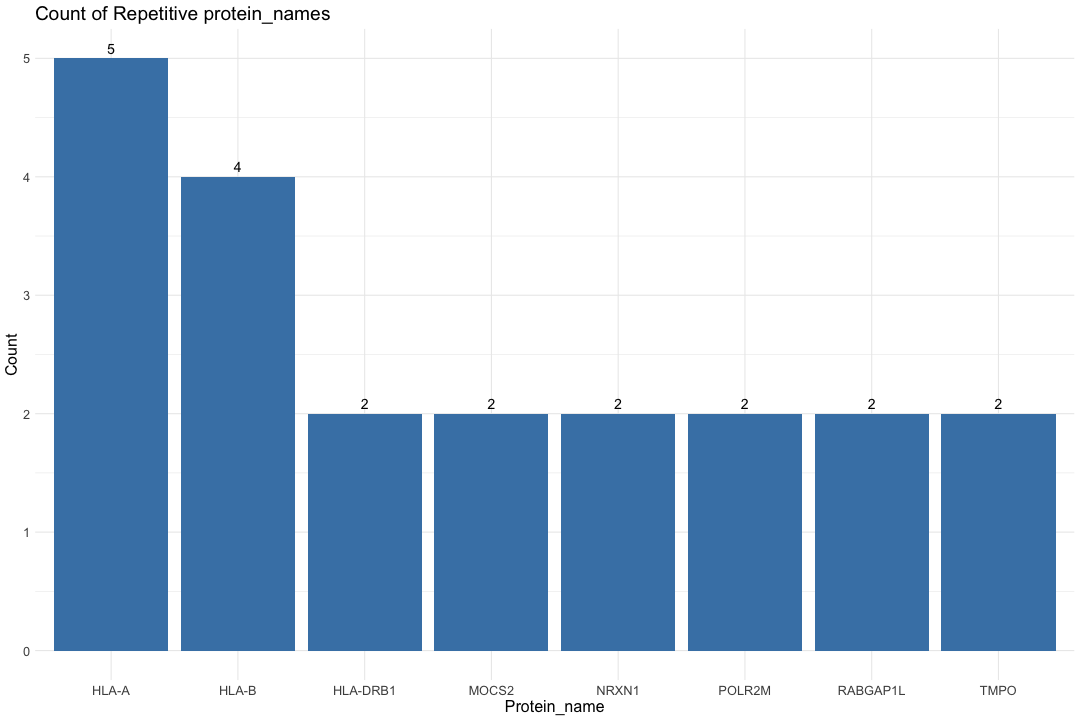
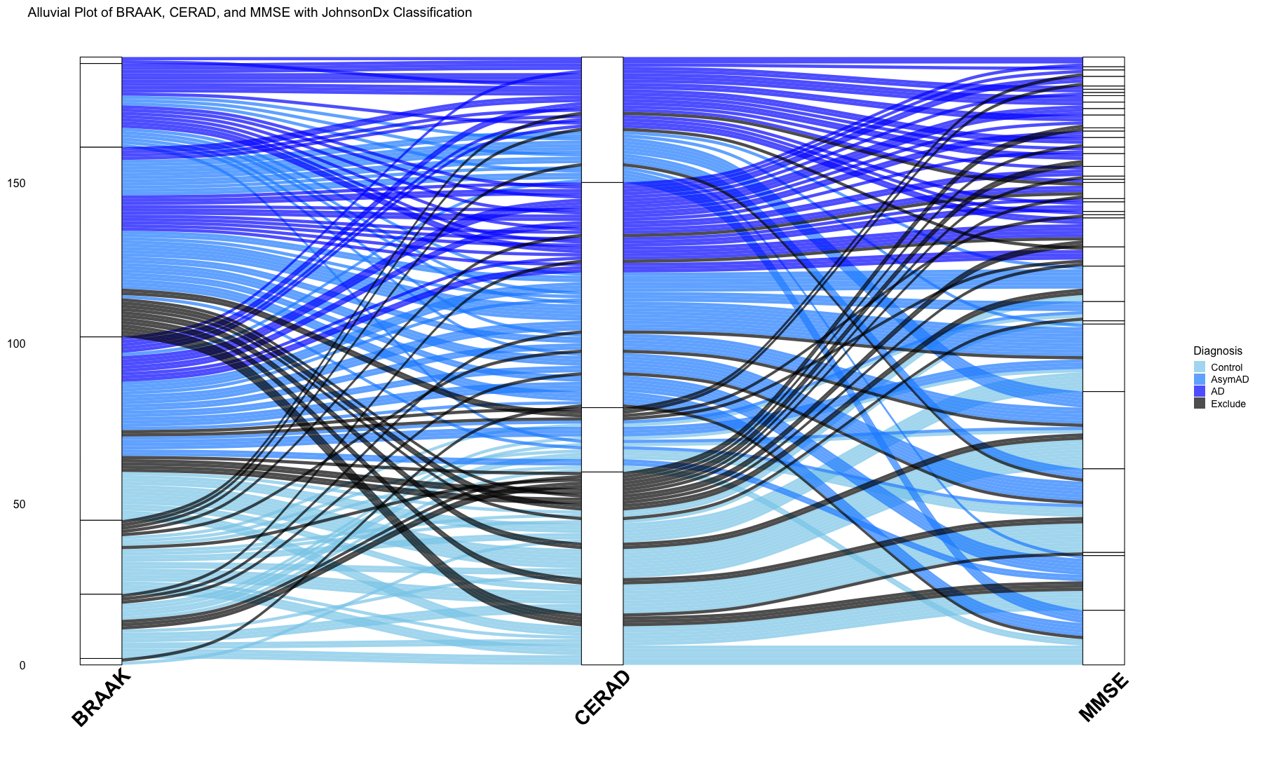
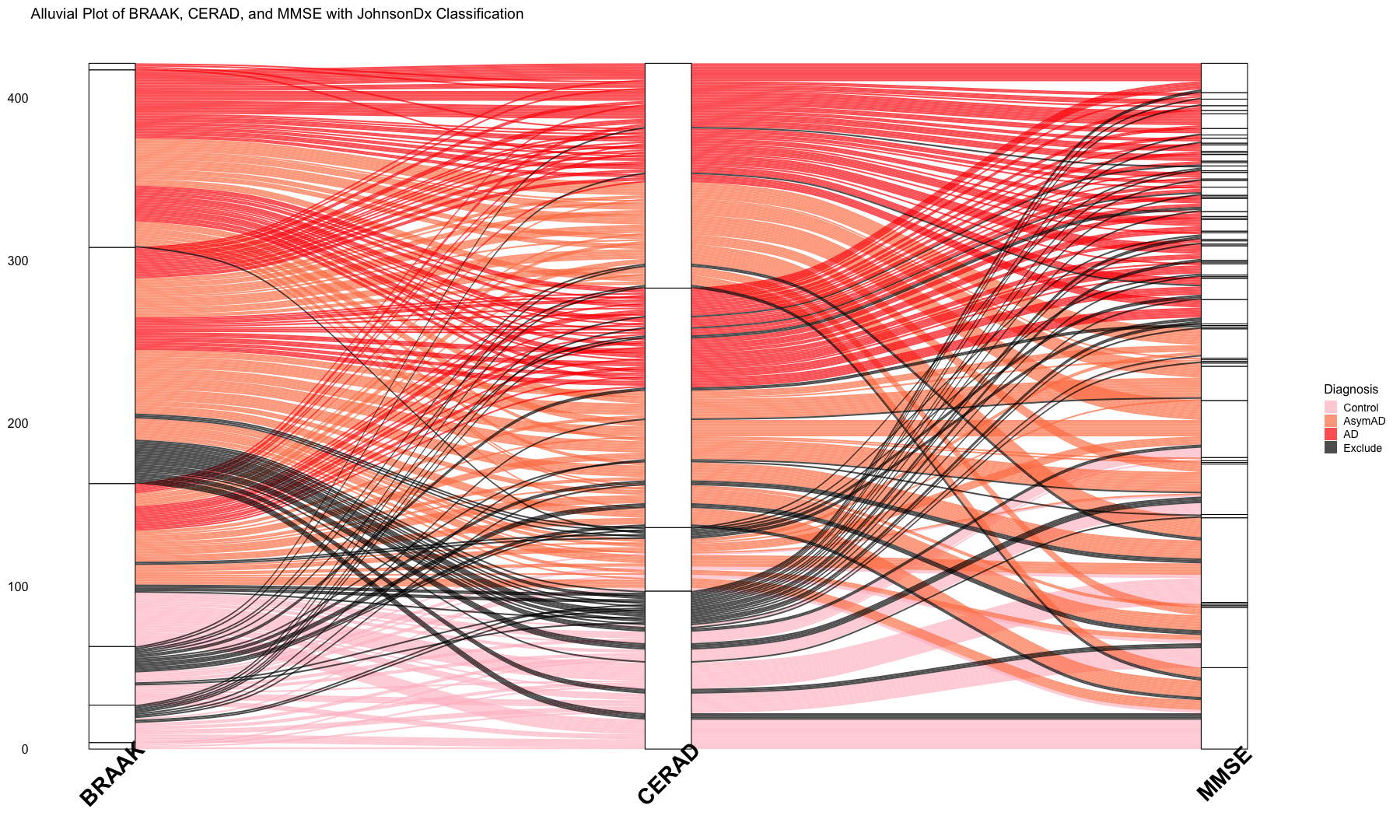
# Alluvial plots implemented here to visualize frequency distributions of braaksc, CERAD and MMSE stages over the diagnosis catagories
library(ggalluvial)
# Create a subset of the DLPFC sample description file with male samples only
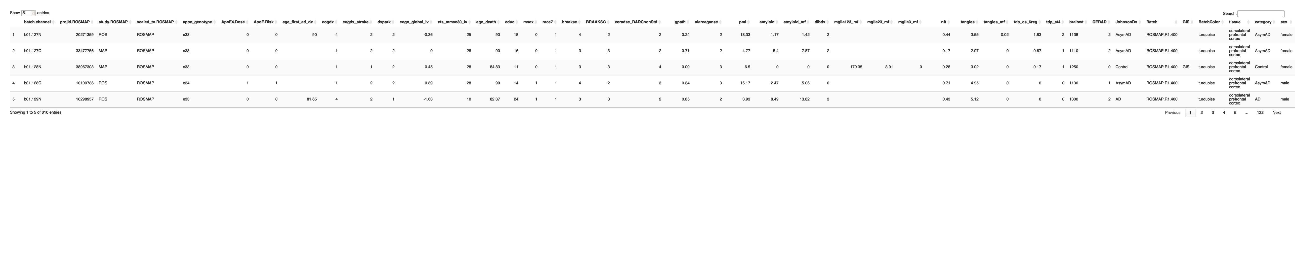
sample_data_DLPFC_male <- protein_metadata_ROSMAP[protein_metadata_ROSMAP$sex == "male", ]
# Create a subset of the DLPFC sample description file with female samples only
sample_data_DLPFC_female <- protein_metadata_ROSMAP[protein_metadata_ROSMAP$sex == "female", ]
## Male
# Prepare the data for the alluvial plot
sample_data_DLPFC_male <- sample_data_DLPFC_male %>%
mutate(
BRAAK = factor(BRAAKSC, levels = sort(unique(BRAAKSC))),
CERAD = factor(ceradsc_RADCnonStd, levels = sort(unique(ceradsc_RADCnonStd))),
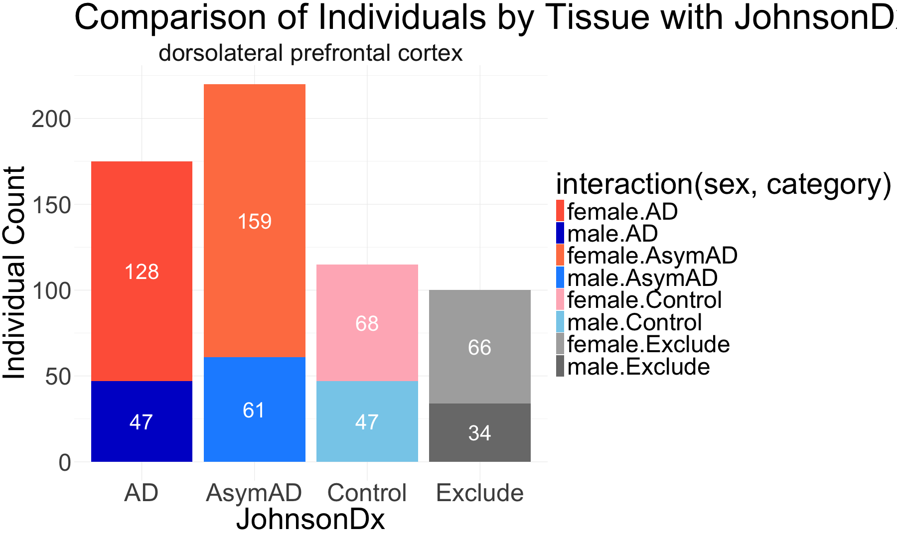
JohnsonDx = factor(category, levels = c("Control", "AsymAD", "AD", "Exclude"))
)
# Create the plot with the updated intervals and proper labels
ggplot(sample_data_DLPFC_male,
aes(
axis1 = BRAAK,
axis2 = CERAD,
axis3 = cts_mmse30_lv,
fill = JohnsonDx
)) +
geom_alluvium(aes(fill = JohnsonDx), alpha = 0.7, width = 1/12) + # Ribbons
geom_stratum(fill = "white", color = "black", width = 1/12) + # Stratum rectangles in white
scale_fill_manual(
values = c("Control" = "skyblue", "AsymAD" = "dodgerblue", "AD" = "blue", "Exclude" = "black")
) +
labs(
title = "Alluvial Plot of BRAAK, CERAD, and MMSE with JohnsonDx Classification",
x = "",
y = "Count",
fill = "Diagnosis"
) +
theme_classic(base_size = 16) +
theme(
axis.line = element_blank(),
axis.ticks = element_blank(),
axis.text = element_blank(),
axis.title = element_blank(),
axis.text.x = element_blank(), # Remove X-axis text
axis.ticks.x = element_blank(), # Remove X-axis ticks
axis.title.x = element_blank(), # Remove X-axis title
axis.text.y = element_text(size = 16),
legend.text = element_text(size = 14),
legend.title = element_text(size = 16),
plot.margin = margin(t = 10, r = 10, b = 40, l = 10) # Extra space for labels
) +
annotate("text", x = 1, y = -10, label = "BRAAK", size = 10, fontface = "bold", angle = 45) +
annotate("text", x = 2, y = -10, label = "CERAD", size = 10, fontface = "bold", angle = 45) +
annotate("text", x = 3, y = -10, label = "MMSE", size = 10, fontface = "bold", angle = 45)